Erlang GraphQL Tutorial
The guide here is a running example of an API implemented in Erlang through the ShopGun GraphQL engine. The API is a frontend to a database, containing information about the Star Wars films by George Lucas. The intent is to provide readers with enough information they can go build their own GraphQL servers in Erlang.
We use the GraphQL system at https://shopgun.com as a data backend. We sponsor this tutorial as part of our Open Source efforts. We developed this GraphQL system to meet our demands as our system evolves. The world of tracking businesses and offers is a highly heterogeneous dataset, which requires the flexibility of something like GraphQL.
Because GraphQL provides a lot of great tooling, we decided to move forward and implement a server backend for Erlang, which didn’t exist at the time.
At the same time, we recognize other people may be interested in the system and its development. Hence the decision was made to open source the GraphQL parts of the system.
Introduction
The Erlang GraphQL system allows you to implement GraphQL servers in Erlang. It works as a library which you can use on top of existing web servers such as Cowboy, Webmachine, Yaws and so on.
As a developer, you work by providing a schema which defines the query structure which your server provides. Next, you map your schema unto Erlang modules which then defines a binding of the two worlds.
Clients execute queries to the server according to the structure of the schema. The GraphQL system then figures out a query plan for the query and executes the query. This in turn calls your bound modules and this allows you to process the query, load data, and so on.
For a complete list of changes over time to this document, take a look at the Changelog appendix.
On this tutorial
| We are currently building the document and are still making changes to it. Things can still move around and change. If you see a “TBD” marker it means that section is “To Be Done” and will be written at a later point. In the same vein, the code base is being built up as well, so it may not be that everything is fully described yet. |
| The current version of Erlang GraphQL returns some errors which are hard to parse and understand. It is our intention to make the error handling better and more clean in a later version. |
The tutorial you are now reading isn’t really a tutorial per se where you type in stuff and see the output. There is a bit too much code for that kind of exposition. Rather, the tutorial describes a specific project implemented by means of the GraphQL system. You can use the ideas herein to build your own.
There are examples of how things are built however, so you may be able to follow along and check out the construction of the system as a whole. Apart from being a small self-contained functional GraphQL project, it is also a small self-contained functional rebar3 project. So there’s that.
Prerequisites
Some Erlang knowledge is expected for reading this guide. General Erlang concept will not be explained, but assumed to be known. Some Mnesia knowledge will also help a bit in understanding what is going on, though if you know anything about databases in general, that is probably enough. Furthermore, some knowledge of the web in general is assumed. We don’t cover the intricacies of HTTP 1.1 or HTTP/2 for instance.
This tutorial uses a couple of dependencies:
-
Rebar3 is used to build the software
-
Cowboy 1.x is used as a web server for the project
-
GraphiQL is used as a web interface to the Graph System
-
Erlang/OTP version 19.3.3 was used in the creation of this tutorial
Supported Platforms
The GraphQL system should run on any system which can run Erlang. The library does not use any special tooling, nor does it make any assumptions about the environment. If Erlang runs on your platform, chances are that GraphQL will too.
Comments & Contact
The official repository location is
If you have comments on the document or corrections, please open an Issue in the above repository on the thing that is missing. Also, feel free to provide pull requests against the code itself.
Things we are particularly interested in:
-
Parts you don’t understand. These often means something isn’t described well enough and needs improvement.
-
Code sequences that doesn’t work for you. There is often some prerequisite the document should mention but doesn’t.
-
Bad wording. Things should be clear and precise. If a particular sentence doesn’t convey information clearly, we’d rather rewrite it then confuse the next reader.
-
Bugs in the code base.
-
Bad code structure. A problem with a tutorial repository is that it can “infect” code in the future. People copy from this repository, so if it contains bad style, then that bad style is copied into other repositories, infecting them with the same mistakes.
-
Stale documentation. Parts of the documentation which were relevant in the past but isn’t anymore. For instance ID entries which doesn’t work anymore.
License
Copyright © 2017 ShopGun.
Licensed under the Apache License, Version 2.0 (the "License"); you may not use this file except in compliance with the License. You may obtain a copy of the License at
http://www.apache.org/licenses/LICENSE-2.0
Unless required by applicable law or agreed to in writing, software distributed under the License is distributed on an "AS IS" BASIS, WITHOUT WARRANTIES OR CONDITIONS OF ANY KIND, either express or implied. See the License for the specific language governing permissions and limitations under the License.
Acknowledgments
-
Everyone involved in the Star Wars API. We use that data extensively.
-
The GraphQL people who did an excellent job at answering questions and provided us with a well-written specification.
-
Josh Price. The parser was derived from his initial work though it has been changed a lot since the initial commit.
Why GraphQL
A worthy question to ask is “Why GraphQL?”
GraphQL is a natural extension of what we are already doing on the Web. As our systems grow, we start realizing our systems become gradually more heterogeneous in the sense that data becomes more complex and data gets more variance.
In addition—since we usually have a single API serving multiple different clients, written in different languages for different platforms—we need to be flexible in query support. Clients are likely to evolve dynamically, non-linearly, and at different paces. Thus, the backend must support evolution while retaining backwards compatibility. Also, we must have a contract or protocol between the clients and the server that is standardized. Otherwise, we end up inventing our own system again and again, and this is a strenuous affair which has little to no reuse between systems.
The defining characteristic of GraphQL is that the system is client-focused and client-centric. Data is driven by the client of the system, and not by the server. The consequence is that the delivery-time for features tend to be shorter. As soon as the product knows what change to make, it can often be handled with less server-side interaction than normally. Especially for the case where you are recombining existing data into a new view.
RESTful APIs have served us well for a long time. And they are likely to continue serving as well in a large number of situations. However, if you have a system requiring more complex interaction, chances are you are better off by taking the plunge and switching your system to GraphQL.
RESTful APIs recently got a powerful improvement in HTTP/2 which allows RESTful APIs to pipeline far better than what they did earlier. However, you still pay the round trip time between data dependencies in an HTTP/2 setting: You need the listing of keys before you can start requesting the data objects on those keys. In contrast, GraphQL queries tend to be a single round-trip only. A full declarative query is formulated and executed, without the need of any intermediate query. This means faster response times. Even in the case where a single query becomes slower since there is no need for followup queries.
A major (subtle) insight is that in a GraphQL server, you don’t have to hand-code the looping constructs which tend to be present in a lot of RESTful APIs. To avoid the round-trip describes in the preceding paragraph, you often resolve to a solution where a specialized optimized query is constructed and added to the system. This specialized endpoint is then looping over the data in one go so you avoid having to do multiple round-trips.
In a GraphQL system, that looping is handled once-and-for-all by the GraphQL engine. You are only implementing callbacks that run as part of the loop. A lot of tedious code is then handled by GraphQL and we avoid having to code this again and again for each RESTful web service we write.
You can often move your system onto GraphQL a bit at a time. You don’t
have to port every endpoint in the beginning. Often, people add some
kind of field, previousId say, which is used as an identifier in the
old system. Then you can gradually take over data from an old system
and port it on top of GraphQL. Once the ball is rolling, it is likely
that more and more clients want to use it, as it is a easier interface
for them to use.
System Tour
Since a system as large as GraphQL can seem incomprehensible when you first use it, we will begin by providing a system tour explaining by example how the system works. In order to start the system for the first time, we must construct a release.
To make a release, run the following command:
$ make releaseThis builds a release inside the _build directory and makes it
available. In order to run the release, we can ask to run it with a
console front-end, so we get a shell on the Erlang system:
$ _build/default/rel/sw/bin/sw consoleThe system should boot and start running. A typical invocation looks like:
Erlang/OTP 19 [erts-8.3] [source] [64-bit] [smp:8:8] [async-threads:30] [hipe] [kernel-poll:true] [dtrace]

15:33:05.705 [info] Application lager started on node 'sw@127.0.0.1'
15:33:05.705 [info] Application ranch started on node 'sw@127.0.0.1'
15:33:05.706 [info] Application graphql started on node 'sw@127.0.0.1'
15:33:05.706 [info] Application sw_core started on node 'sw@127.0.0.1'
15:33:05.706 [info] Application cowboy started on node 'sw@127.0.0.1'
15:33:05.706 [info] Starting HTTP listener on port 17290
Eshell V8.3  (abort with ^G)
(sw@127.0.0.1)1>
To exit an Erlang node like this, you can either Ctrl-C twice
which stops the system abruptly. Or you can be nice to the system and
ask it to close gracefully one application at a time by entering
q().<RET> in the shell.
|
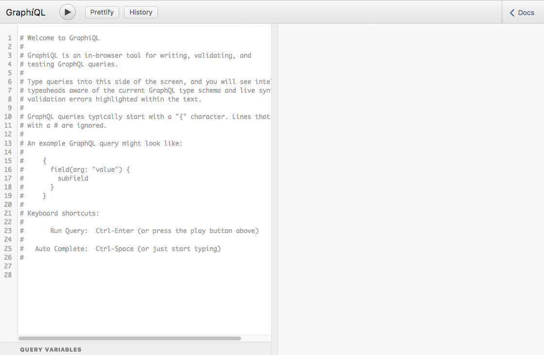
Once the Erlang emulator is running our sw release, we can point a
browser to http://localhost:17290/ and you should be greeted
with the following screen:
First query
The first query we will run requests a given Planet from the system. This query follows a set of rules, the Relay Modern GraphQL conventions. These conventions are formed by Facebook as part of their Relay Modern system. It defines a common set of functionality on top of the GraphQL system which clients can rely on.
In particular, our first query uses the rules of Object Identification which is a way to load an object for which you already know its identity. A more complete exposition of the conventions are in the section Relay Modern, but here we skip the introduction for the sake of brevity:
query PlanetQuery {
  node(id:"UGxhbmV0OjE=") { (1)
    ... on Planet { (2)
      id (3)
      name
      climate
    }
  }
}| 1 | The ID entered here is opaque to the client, and we assume it was obtained in an earlier query. We will show typical ways to list things later in this section. |
| 2 | This notation, if you are only slightly familiar with GraphQL is
called an inline fragment. The output of the node field is of
type Node and here we restrict ourselves to the type Planet. |
| 3 | This requests the given fields in the particular planet we loaded. |
If you enter this in the GraphiQL left window and press the “Run” button, you should get the following response:
{
  "data": {
    "node": {
      "climate": "arid",
      "id": "UGxhbmV0OjE=",
      "name": "Tatooine"
    }
  }
}
Note how the response reflects the structure of the query. This is a powerful feature of GraphQL since it allows you to build up queries client side and get deterministic results based off of your query-structure.
More advanced queries
Let us look at a far more intricate query. In this query, we will also request a planet, but then we will ask “what films does this planet appear in?” and we will ask “Who are the residents on the planet?”--who has the planet as their homeworld?.
To do this, we use pagination. We ask for the first 2 films and the first 3 residents. We also ask for the relevant meta-data of the connections as we are here:
query Q {
  node(id:"UGxhbmV0OjE=") {
    ... on Planet {
      id
      name
      climate
      filmConnection(first: 2) {
        totalCount
        pageInfo {
          hasNextPage
          hasPreviousPage
        }
        edges {
          node {
            ...Films
          }
          cursor
        }
      }
      residentConnection(first: 3) {
        totalCount
        pageInfo {
          hasNextPage
          hasPreviousPage
        }
        edges {
          node {
            ...Residents
          }
          cursor
        }
      }
    }
  }
}

fragment Films on Film {
  id
  title
  director
}

fragment Residents on Person {
  id
  name
  gender
}
The fragment parts allows your queries to re-use different subsets
of a larger query again and again. We use this here to show off that
capability of GraphQL. The result follows the structure of the query:
{
  "data": {
    "node": {
      "climate": "arid",
      "filmConnection": {
        "edges": [
          {
            "cursor": "MQ==",
            "node": {
              "director": "George Lucas",
              "id": "RmlsbTox",
              "title": "A New Hope"
            }
          },
          {
            "cursor": "Mg==",
            "node": {
              "director": "Richard Marquand",
              "id": "RmlsbToz",
              "title": "Return of the Jedi"
            }
          }
        ],
        "pageInfo": {
          "hasNextPage": true,
          "hasPreviousPage": false
        },
        "totalCount": 5
      },
      "id": "UGxhbmV0OjE=",
      "name": "Tatooine",
      "residentConnection": {
        "edges": [
          {
            "cursor": "MQ==",
            "node": {
              "gender": "n/a",
              "id": "UGVyc29uOjg=",
              "name": "R5-D4"
            }
          },
          {
            "cursor": "Mg==",
            "node": {
              "gender": "male",
              "id": "UGVyc29uOjEx",
              "name": "Anakin Skywalker"
            }
          },
          {
            "cursor": "Mw==",
            "node": {
              "gender": "male",
              "id": "UGVyc29uOjE=",
              "name": "Luke Skywalker"
            }
          }
        ],
        "pageInfo": {
          "hasNextPage": true,
          "hasPreviousPage": false
        },
        "totalCount": 10
      }
    }
  }
}
Simple Mutations
Now, let us focus on altering the database through a mutation. In GraphQL, this is the way a client runs “stored procedures” on the Server side. The Star Wars example has tooling for factions in the Star Wars universe, but there are currently no factions defined. Let us amend that by introducing the rebels:
mutation IntroduceFaction($input: IntroduceFactionInput!) {
  introduceFaction(input: $input) {
    clientMutationId
    faction {
      id
      name
      ships {
        totalCount
      }
    }
  }
}
This query uses the GraphQL feature of input variables. In the UI, you can click and expand the section Query Variables under the query pane. This allows us to build a generic query like the one above and then repurpose it for creating any faction by providing the input variables for the query:
{
  "input": {
    "clientMutationId": "D9A5939A-DF75-4C78-9B32-04C1C64F9D9C", (1)
    "name": "Rebels"
  }
}| 1 | This is chosen arbitrarily by the client and can be any string. Here we use an UUID. |
The server, when you execute this query, will respond with the creation of a new Faction and return its id, name and starships:
{
  "data": {
    "introduceFaction": {
      "clientMutationId": "D9A5939A-DF75-4C78-9B32-04C1C64F9D9C", (1)
      "faction": {
        "id": "RmFjdGlvbjoxMDAx", (2)
        "name": "Rebels",
        "ships": {
          "totalCount": 0 (3)
        }
      }
    }
  }
}| 1 | The server reflects back the unique client-generated Id for correlation purposes. |
| 2 | The Id migth be different depending on how many Faction objects you created. |
| 3 | We have yet to assign any starships to the faction, so the count is currently 0. |
We can now query this faction by its Id because it was added to the system:
query FactionQuery {
  node(id: "RmFjdGlvbjoxMDAx") {
     ... on Faction {
       id
       name
     }
  }
}
The system also persisted the newly created faction in its database so restarting the system keeps the added faction.
Use q() in the shell to close the system gracefully.
Otherwise you may be in a situation where a change isn’t reflected on
disk. The system will still load a consistent view of the database,
but it will be from before the transaction were run. The Mnesia system
used is usually quick at adding data to its WAL, but there is no
guarantee.
|
More complex mutations
With the rebels in the Graph, we can now create a new Starship, a B-Wing, which we will add to the graph. We will also attach it to the newly formed faction of Rebels. The mutation here exemplifies operations in which you bind data together in GraphQL. Our mutation looks like:
mutation IntroduceBWing {
  introduceStarship(input:
    { costInCredits: 5.0, (1)
      length: 20.0,
      crew: "1",
      name: "B-Wing",
      faction: "RmFjdGlvbjoxMDAx", (2)
      starshipClass: "fighter"}) {
    starship {
      id
      name
    }
    faction {
      id
      name
      ships {
        totalCount

        edges {
          node {
            id name
          }
        }
      }
    }
  }
}| 1 | The values here are not for a “real” B-wing fighter, but are just made up somewhat arbitrarily. |
| 2 | The ID of the Faction. If you run this the ID may be a bit different so make sure you get the right ID here. |
We create a new Starship, a B-wing, in the Rebels faction. Note the resulting object, IntroduceStarshipPayload, contains the newly created Starship as well as the Faction which was input as part of the query. This is common in GraphQL: return every object of interest as part of a mutation.
The result of the query is:
{
  "data": {
    "introduceStarship": {
      "faction": {
        "id": "RmFjdGlvbjoxMDAx",
        "name": "Rebels",
        "ships": {
          "edges": [
            {
              "node": {
                "id": "U3RhcnNoaXA6MTAwMQ==",
                "name": "B-Wing"
              }
            }
          ],
          "totalCount": 1
        }
      },
      "starship": {
        "id": "U3RhcnNoaXA6MTAwMQ==",
        "name": "B-Wing"
      }
    }
  }
}
Note how the newly formed starship is now part of the Rebel factions
starships, and that the total count of starships in the Faction is now
1. The created field on the Starship is automatically generated by
the system as part of introducing it.
Note: Not all the fields on the newly formed starship are "valid" insofar we decided to reduce the interface here in order to make it easier to understand in the tutorial. A more complete solution would force us to input every field on the Starship we just introduced and also use sensible defaults if not given.
This tutorial
This tutorial will tell you how to create your own system which can satisfy queries as complex and complicated as the examples we just provided. It will explain the different parts of the GraphQL system and how you achieve the above.
Getting Started
This tutorial takes you through the creation of a GraphQL server implementing the now ubiquitous Star Wars API. This API was created a couple of years ago to showcase a REST interface describing good style for creation of APIs. The system revolves around a database containing information about the Star Wars universe: species, planets, starships, people and so on.
GraphQL, when it was first released, ported the Star Wars system from REST to GraphQL in order to showcase how an API would look once translated. Because of its ubiquity, we have chosen to implement this schema in the tutorial you are now reading:
-
It is a small straightforward example. Yet it is large enough that it will cover most parts of GraphQL.
-
If the reader is already familiar with the system in another GraphQL implementation, it makes pickup of Erlang GraphQL faster.
-
We can use a full system as a driving example for this tutorial.
-
If Erlang GraphQL has a bug, it may be possible to showcase the bug through this repository. This makes it easier to work on since you have immediate common ground.
The goal of the tutorial is to provide a developer with a working example from which you can start. Once completed, you can start adding your own types to the tutorial. And once they start working, you can "take over" the system and gradually remove the Star Wars parts until you have a fully working example.
This implementation backs the system by means of a Mnesia database. The choice is deliberate for a couple of reasons:
-
Mnesia is present in any Erlang system and thus it provides a simple way to get started and setup.
-
Mnesia is not a Graph Database. This makes it explicit your database can be anything. In fact, the "Graph" in GraphQL is misnomer since GraphQL works even when your data does not have a typical Graph-form. It is simply a nice query structure.
What we do not cover
This tutorial doesn’t cover everything in the repository:
-
The details of the
rebar3integration and therelxrelease handling. -
The tutorial only covers the parts of the code where there is something to learn. The areas of the code getting exposition in this document is due to the fact that they convey some kind of important information about the use of the GraphQL system for Erlang. Other parts, which are needed for completeness, but aren’t as important are skipped.
-
There is no section on “how do I set up an initial Erlang environment” as it is expected to be done already.
Overview
The purpose of a GraphQL server is to provide a contract between a client and a server. The contract ensures that the exchange of information follows a specific structure, and that queries and responses are in accordance with the contract specification.
Additionally, the GraphQL servers contract defines what kind of queries are possible and what responses will look like. Every query and response is typed and a type checker ensures correctness of data.
Finally, the contract is introspectable by the clients. This allows automatic deduction of queries and built-in documentation of the system interface.
Thus, a GraphQL server is also a contract checker. The GraphQL system ensures that invalid queries are rejected, which makes it easier to implement the server side: you can assume queries are valid to a far greater extent than is typical in other systems such as typical REST interfaces.
Plan
In order to get going, we need a world in which to operate. First, we must provide two schemas: one for the GraphQL system, and one for the Mnesia database.
The GraphQL schema defines the client/server contract. It consists of several GraphQL entity kinds. For example:
-
Scalar types—Extensions on top of the default types. Often used for Dates, DateTimes, URIs, Colors, Currency, Locales and so on.
-
Enumerations—Values taken from a limited set. An example could be the enumeration of weekdays: “MONDAY, TUESDAY, WEDNESDAY, …, SUNDAY”.
-
Input Objects—Data flowing from the Client to the Server (Request).
-
Output Objects—Data flowing from the Server to the Client (Response).
A somewhat peculiar choice by the GraphQL authors is that the world of Input and Output objects differ. In general, a Client has no way to "PUT" an input object back into the Graph as is the case in REST systems. From a type-level perspective, client requests and server responses have different polarity.
It may seem as if this is an irritating choice. You often have to specify the “same” object twice: once for input and once for output. However, as your GraphQL systems grows in size, it turns out this choice is the right one. You quickly run into situations where a client supplies a desired specific change where many of the fields on the output object doesn’t make sense. By splitting the input and output world, it is easy to facilitate since the input objects can omit many fields that doesn’t make sense.
In a way, your GraphQL system is built such that changes to the data is done by executing “transactions” through a set of stored procedures. This can be seen as using the "`PATCH`" method of RESTful interfaces and not having a definition of PUT.
GraphQL splits the schema into two worlds: query and mutation. The difference from the server side is mostly non-existent: the GraphQL system is allowed to parallelize queries but not mutations. But from the perspective of the client, the starting points in the graph is either the query or the mutation object.
GraphQL implements what is essentially CQRS by making a distinction between the notion of a query and a mutation. Likewise, the server side makes this distinction. But on the server side it is merely implemented by having different starting objects in the graph execution.
Our Star Wars schema uses the database Mnesia as a backend. It is important to stress that you often have a situation where your database backend doesn’t map 1-1 onto your specified GraphQL schema. In larger systems, this is particularly important: the GraphQL schema is often served by multiple different backends, and those backends are not going to cleanly map onto the world we expose to the clients. So the GraphQL schema contract becomes a way to mediate between the different data stores. As an example, you may satisfy some parts of the GraphQL query from a dedicated search system—such as ElasticSearch—while others are served as rows from a traditional database, such as MySQL or Postgresql. You may even have a message queue broker or some other subsystem in which you have relevant data you want to query. Or perhaps, some queries are handled by micro-services in your architecture.
Over the course of having built larger systems, we’ve experienced that mappings which tries to get isomorphism between the backend and the schema creates more problems than they solve. Small changes have consequence in all of the stack. Worse, you can’t evolve part of the system without evolving other parts which impairs the flexibility of the system.
Another problem is that you may end up with an impedance mismatch between the Objects and links of the GraphQL query and the way you store your data in the backend. If you force a 1-1 relationship between the two, you can get into trouble because your GraphQL schema can’t naturally describe data.
A common problem people run into with Mnesia is how to “get started”. What people often resort to are solutions where an initial database is created if it doesn’t exist. These solutions are often brittle.
Here, we pick another solution. A helper can create a database schema for us, with all the necessary tables. The real release assumes the presence of an initial database and won’t boot without one. This means the Erlang release is simpler. There is always some database from which it can boot and operate. That database might be the empty database since we are just starting out. But in particular, the release won’t concern itself with creating an initial database. Rather it will assume one is already existing.
The situation is not much different than using a traditional schema-oriented database. Usually, you have to create the database first, and then populate the schema with some initial data. It is just because of Rails/Django like systems in which databases are migrate-established, we’ve started using different models.
Mnesia
Setting up an initial Mnesia schema
To get up and running, we begin by constructing a Mnesia schema we can start from. We do this by starting a shell on the Erlang node and then asking it to create the schema:
$ git clean -dfxq (1)
$ make compile (2)
$ make shell-schema (3)
erl -pa `rebar3 path` -name sw@127.0.0.1
Erlang/OTP 19 [erts-8.3] [source] [64-bit] [smp:8:8] [async-threads:10] [hipe] [kernel-poll:false] [dtrace]

Eshell V8.3  (abort with ^G)
1> sw_core_db:create_schema(). % (4)| 1 | Clean out the source code repository to make sure there is no lingering files: Caution when using this command as it could potentially delete files if used in wrong directory. |
| 2 | Compile the code so we have compiled versions of modules we can loaded |
| 3 | Run the Erlang interpreter with an altered path for our newly compiled modules |
| 4 | Create the schema |
The call create_schema() runs the following schema creation code:
create_schema() ->
    mnesia:create_schema([node()]),
    application:ensure_all_started(mnesia),
    ok = create_fixture(disc_copies, "fixtures"),
    mnesia:backup("FALLBACK.BUP"),
    mnesia:install_fallback("FALLBACK.BUP"),
    application:stop(mnesia).

create_fixture(Type, BaseDir) ->
    ok = create_tables(Type),
    ok = populate_tables(BaseDir),
    ok.
Creating the schema amounts to running a set of commands from the Mnesia documentation. The helper function to create tables contains a large number of tables, so we are just going to show two here:
create_tables(Type) ->
    {atomic, ok} =
        mnesia:create_table(
          starship,
          [{Type, [node()]},
           {type, set},
           {attributes, record_info(fields, starship)}]),
    {atomic, ok} =
        mnesia:create_table(
          species,
          [{Type, [node()]},
           {type, set},
           {attributes, record_info(fields, species)}]),
In Mnesia, tables are Erlang records. The #planet{} record needs
definition and is in the header file sw_core_db.hrl. We simply list
the entries which are defined the SWAPI GraphQL schema so we can store
the concept of a planet in the system:
-record(planet,
        {id :: integer(),
         edited :: calendar:datetime(),
         climate :: binary(),
         surface_water :: integer(),
         name :: binary(),
         diameter :: integer(),
         rotation_period :: integer(),
         created :: calendar:datetime(),
         terrains :: [binary()],
         gravity :: binary(),
         orbital_period :: integer() | nan,
         population :: integer() | nan
}).
Every other table in the system is handled in the same manner, but are not given here for brevity. They follow the same style as the example above.
Populating the database
Once we have introduced tables into the system, we can turn our
attention to populating the database tables. For this, we use the
SWAPI data set as the primary data source. This set has its fixtures
stored as JSON document. So we use jsx to decode those JSON
documents and turn them into Mnesia records, which we then insert into
the database.
We can fairly easily write a transformer function which take the JSON
terms and turn them into appropriate Mnesia records. Planets live in a
fixture file planets.json, which we can read and transform. Some
conversion is necessary on the way since the internal representation
differ slightly from the representation in the fixture:
json_to_planet(
  #{ <<"pk">> := ID,
     <<"fields">> := #{
         <<"edited">> := Edited,
         <<"climate">> := Climate,
         <<"surface_water">> := SWater,
         <<"name">> := Name,
         <<"diameter">> := Diameter,
         <<"rotation_period">> := RotationPeriod,
         <<"created">> := Created,
         <<"terrain">> := Terrains,
         <<"gravity">> := Gravity,
         <<"orbital_period">> := OrbPeriod,
         <<"population">> := Population
        }}) ->
    #planet {
       id = ID,
       edited = datetime(Edited),
       climate = Climate,
       surface_water = number_like(SWater),
       name = Name,
       diameter = number_like(Diameter),
       rotation_period = number_like(RotationPeriod),
       created = datetime(Created),
       terrains = commasplit(Terrains),
       gravity = Gravity,
       orbital_period = number_like(OrbPeriod),
       population = number_like(Population)
}.
Once we have this function down, we can utilize it to get a list of Mnesia records, which we can then insert into the database through a transaction:
populate_planets(Terms) ->
    Planets = [json_to_planet(P) || P <- Terms],
    Txn = fun() ->
                  [mnesia:write(P) || P <- Planets],
                  ok
          end,
    {atomic, ok} = mnesia:transaction(Txn),
    ok.
The code to read in and populate the database is fairly straightforward. It is the last piece of the puzzle to inject relevant data into the Mnesia database:
populate(File, Fun) ->
    {ok, Data} = file:read_file(File),
    Terms = jsx:decode(Data, [return_maps]),
    Fun(Terms).

populate_tables(BaseDir) ->
    populate(filename:join(BaseDir, "transport.json"),
             fun populate_transports/1),
    populate(filename:join(BaseDir, "starships.json"),
             fun populate_starships/1),
    populate(filename:join(BaseDir, "species.json"),
             fun populate_species/1),
    populate(filename:join(BaseDir, "films.json"),
             fun populate_films/1),
    populate(filename:join(BaseDir, "people.json"),
             fun populate_people/1),
    populate(filename:join(BaseDir, "planets.json"),
             fun populate_planets/1),
    populate(filename:join(BaseDir, "vehicles.json"),
             fun populate_vehicles/1),
    setup_sequences(),
    ok.
This creates a fixture in the database such that when we boot the database, the planets, transports, people, …, will be present in the Mnesia database when we boot the system.
Creating a FALLBACK for the database
Once we have run the schema creation routine, a file called
FALLBACK.BUP is created. We copy this to the database base core in
the repository
$ cp FALLBACK.BUP db/FALLBACK.BUPwhich makes the empty schema available for the release manager of the
Erlang system. When we cook a release, we will make sure to copy this
initial schema into the correct Mnesia-directory of the release.
Because the file is named FALLBACK.BUP, it is a fallback backup file.
This will “unpack” itself to become a new empty database as if you
had rolled in a backup on the first boot of the system. Thus we avoid
our system having to deal with this problem at start up.
A real system will override the location of the Mnesia dir
parameter and define a separate directory from which the Mnesia
database will run. Initially, the operator will place the
FALLBACK.BUP file in this directory to get going, but once we are
established, and people start adding in data, we can’t reset anything
when deploying new versions. Hence the separate directory so we can
upgrade the Erlang system without having to protect the database as
much.
|
We now have the ability to create new database tables easily and we have a Mnesia database for backing our data. This means we can start turning our attention to the GraphQL schema.
GraphQL Schema
With a Mnesia database at our disposal, we next create a GraphQL schema definition. This file describes the contract between the client system and the server system. It is used by the GraphQL system to know which queries are valid and which aren’t.
In accordance with OTP design principles, we place this schema inside
a projects priv directory. Our GraphQL system can then refer to the
private directory of the application in order to load this schema when
the system boots up.
Identity encoding
In GraphQL, you have a special type, ID, which is used to attach an identity to objects. It is typically used as a globally unique identifier for each object in the graph. Even across different object types; no two objects share a ID, even if they are of different type.
The ID is always generated by the server. Hence, a client must only treat an ID as an opaque string value and never parse on the string value. It can only return the ID value back to the server later on.
To make this more obvious, GraphQL implementations usually base64 encode
their ID-values. In Mnesia, our rows IDs will be integers, and they
will overlap between different types/tables in the database. Since IDs
should be globally unique, we use an encoding in GraphQL. The Starship
with id 3 will be encoded as base64("Starship:3"). And the planet
Tatooine taken from the System Tour is encoded as
base64("Planet:1"). This definition somewhat hides the
implementation and also allows the server backend to redefine IDs
later for objects. Another use of the encoding is that it can define
what datasource a given came from, so you can figure out where to find
that object. It is highly useful in migration scenarios.
The encoder is simple because we can assume the server provides valid values:
encode({Tag, ID}) ->
    BinTag = atom_to_binary(Tag, utf8),
    IDStr = integer_to_binary(ID),
    base64:encode(<<BinTag/binary, ":", IDStr/binary>>).
The decoder is a bit more involved. It requires you to fail on invalid inputs. We usually don’t need to know what was invalid. We can simply fail aggressively if things turns out bad. A debugging session will usually uncover the details anyway as we dig into a failure.
decode(Input) ->
    try
        Decoded = base64:decode(Input),
        case binary:split(Decoded, <<":">>) of
            [BinTag, IDStr] ->
                {ok, {binary_to_existing_atom(BinTag, utf8),
                      binary_to_integer(IDStr)}};
            _ ->
                exit(invalid)
        end
    catch
        _:_ ->
            {error, invalid_decode}
    end.
The Node Interface
The Relay Modern specification (see Relay Modern) contains a standard for an Object Identification interface. Our schema implements this standard in order to make integration simpler for clients supporting the standard. The interface, also called the Node interface because of its type, allows you to “start from” any node in the graph which has an id field. That is, every node with identity can be a starting point for a query.
The interface is most often used as a way to refresh objects in a client cache. If the client has a stale object in the cache, and the object has identity, then you can refresh a subset of the graph, setting out from that object.
The interface specification follows the standard closely:
+description(text: "Relay Modern Node Interface")
interface Node {
  +description(text: "Unique Identity of a Node")
  id : ID!
}The Erlang version of GraphQL allows a certain extension by the
Apollo Community @ Github, who are
building tools GraphQL in general. This extension allows you to use
Annotations in GraphQL schemas to attach more information to
particular objects of interest. We use this for documentation. You can
annotate almost anything with +description(text: "documentation")
which in turn attaches that documentation to an entity in the Graph.
Multi-line comments are also possible by using a backtick (`) rather than a quote symbol ("). These allows larger Markdown entries to be placed in the documentation, which tends to be good for documentation of APIs.
| You can’t easily use a backtick (`) inside the multiline quotations. This means you can’t easily write pre-formatted code sections unless you use indentation in the Markdown format. The choice was somewhat deliberate in that there is a workaround currently, and it tends to flow really well when you enter documentation by means of the backtick character. A future version of the parser might redo this decision. |
Object types
We follow the specification for describing object types. Thus, if you
describe an object like a starship as type Starship { … } the
system knows how to parse and internalize such a description. In the
following, we don’t cover all of the schema, but focus on a single
type in order to describe what is going on.
Planets
Since we have planets in the Mnesia database from the previous section, we can define the GraphQL Schema for them as well. The definition is quite straightforward given the Star Wars API we are trying to mimic already contains all the important parts.
For brevity, we omit the documentation of each individual field for now. Though a more complete implementation would probably include documentation on each field to a fine detail.
type Planet implements Node {
  name : String
  diameter : Int
  rotationPeriod : Int
  orbitalPeriod : Int
  gravity : String
  population : Int
  climate : String
  terrains : [String]
  surfaceWater : Int
  filmConnection(after: String, first: Int,
                 before: String, last: Int)
    : PlanetFilmsConnection
  residentConnection(after: String, first: Int,
                     before: String, last: Int)
    : PlanetResidentsConnection
  created : DateTime
  edited : DateTime
  id : ID!
}
Queries & Mutations
Query Object
All GraphQL queries are either a query or a mutation.[1]
Correspondingly, the schema specification contains entries for two
(output) objects, which are commonly called Query and Mutation
respectively. For example, the query object looks like:
type Query {
  +description(text: "Relay Modern specification Node fetcher")
  node(id : ID!) : Node
  +description(text: "Fetch a starship with a given Id")
  starship(id : ID!) : Starship
  allStarships : [Starship]
  allPlanets : [Planet]
  allPeople : [Person]
  allVehicles : [Vehicle]
  allSpecies : [Species]
  allFilms : [Film]
  filmByEpisode(episode: Episode) : Film!
}
The Query object defines the (public) query/read API of your backend. All queries will start from here, and the specification defines what you can do with the given query.
| The introspection capabilities of GraphQL will have the astute reader recognize that this predefined rule of what you can do with a query is very close to automatic discovery of capabilities. In other words, you get close to the notion of Hypertext as the engine of application state, while not reaching it. |
The field node allows you to request any node in the Graph. Later,
we will see how to implement the backend functionality for this call.
In this example, we will request a Starship through the node
interface by first requesting anything implementing the Node
interface, and then use an inline-fragment in order to tell the system
which fields we want to grab inside the starship:
query StarShipQuery($id : ID!) {
    node(id: $id) {
       __typename
       id
       ... on Starship {
          model
          name
       }
    }
}
Fields such as allStarships are in the schema in order to make it
easier to peruse the API. In a real system, such a query would be
dangerous since it potentially allows you to request very large data
sets. In practice you would use pagination or use a search engine to
return such results. Specifically, you would never return all possible
values, but only a subset thereof.
Mutation Object
The Query object concerns itself about reading data. The Mutation object is for altering data. In a CQRS understanding, the Mutation object is the command.
GraphQL treats mutations the same way as queries except for one subtle detail: queries may be executed in parallel on the server side whereas a mutation may not. Otherwise, a mutation works exactly like a query.
Because queries and mutations are the same for the GraphQL engine, we need to build up conventions in the mutation path in order to make things work out. First, since mutations starts off from the Mutation object, we can add fields to that object which isn’t present in the Graph otherwise. This allows us to execute transactions at the server side for changes.
Each transaction becomes a field on the Mutation object. And the
result type of the given field is the return value of the mutation.
This return type, often called the payload contains other objects in
the graph. It allows a client to run a mutation on the server side and
then query on the data it just changed. This corresponds to the
situtation in RESTful models where a POST provides a location:
response header containing the URI of the newly created object. But as
we want to avoid a roundtrip, we “bake” the query into the mutation
in GraphQL.
type Mutation {
  introduceFaction(input: IntroduceFactionInput!)
    : IntroduceFactionPayload
  introduceStarship(input: IntroduceStarshipInput!)
    : IntroduceStarshipPayload
}
Our mutation object grants a client access to a number of commands it
can execute. First, it can create new factions by means of the
introduceFaction field on the object. It can also create a new
Starship through the introduceStarship field.
Both fields take a single parameter, input of a given type (which we
will explain later). It provides data relevant to the given mutation. The
return value is a regular output type in the graph, for instance
IntroduceStarshipPayload:
type IntroduceStarshipPayload {
  clientMutationId : String
  faction : Faction
  starship : Starship
}
It is common that a payload-style object returns every object which
was manipulated as part of the update. In this case, since starship
introduction creates a new starship and refers to a faction, we return
the fields starship and faction. It allows a client to execute
queries pertaining to the current situation. Suppose for example we
add a new starship to a faction. We’d like the starship count of that
faction. This is easy due to the payload object. Factions have a
StarshipConnection, so we can just utilize that to get the count:
mutation IF($input : IntroduceStarshipInput!) {
  introduceStarship(input: $input) {
    starship {
      id
      name
    }
    faction {
      id
      name
      ships {
        totalCount
      }
    }
  }
}
It is typical use to get “cross-talk” updates like this in GraphQL when you refresh objects in the cache, or when you change the data through a mutation.
The mutations given here follow the conventions Facebook has defined for Relay Modern and a further treatment is given in the section Inputs & Payloads.
Input objects
The type system of GraphQL is “moded” as in Prolog/Twelf/Mercury or is “polarized” in the sense of type systems and semantics. Some data has “positive” mode/polarity and flows from the client to the server. Some data has “negative” mode/polarity and flows from the server to the client. Finally, some data are unmoded and can flow in either direction.
GraphQL distinguishes between input and output types. An input is positive and an output is negative. While at first, this might seem like a redundant and bad idea, our experience is that it helps a lot once your system starts to grow.
In GraphQL, the way you should think about Mutations are that they are
“stored procedures” in the backend you can execute. You don’t in
general get access to a command which says “PUT this object back”.
Rather, you get access to a mutation which alters the object in some
predetermined way: favoriteStarship(starshipId: ID!) for instance.
Because of this, GraphQL is built to discriminate between what types of data the client can send and what types of data the server can respond with.
Input and output objects are subject to different rules. In
particular, there is no way to input a null value in an input. The
way a client inputs a no value input is by omission of the input
parameter in question. This choice simplifies clients and servers.
There are times where the client wants to input a number of values at the same time. You could add more parameters to the field:
type Mutation {
    introduceStarship(name: String,
                      class: String,
                      manufacturers: [String], ....)
       : IntroduceStarshipPayload
}
but this often gets unwieldy in the longer run. Rather than this, you can also solve the problem by creating an input object which only works in the input direction:
input IntroduceStarshipInput {
  clientMutationId : String

  name : String
  model : String
  starshipClass : String!
  manufacturers : [String] = [] (1)
  costInCredits : Float!
  length : Float!
  crew : String!

  faction : ID!
}| 1 | Default parameter value, see Schema default values. |
In turn, the client can now input all these values as one. Grouping of like parameters are quite common in GraphQL schemas. Note how input object fields are often vastly different from the output object it corresponds to. This is the reason why having two worlds—input & output—is useful.
| The input object presented here doesn’t contain a full starship input. In a full solution, you would provide means to add in pilots, films, hyperdrive ratings and so on. |
It is possible to define default parameters in the schema as well, as seen in the above example. This is highly useful as a way to simplify the backend of the system. By providing sensible defaults, you can often avoid a specialized code path which accounts for an unknown value. It also simplifies the client as it doesn’t have to input all values unless it wants to make changes from the defaults. Finally it documents, to the client, what the defaults are.
clientMutationId
By now, you have seen that an input object has a clientMutationId
and the corresponding payload also has a clientMutationId. This is
part of Relay Modern conventions.
Every …Input object in a mutation contains a field clientMutationId
which is an optional string. The server reflects the contents of
clientMutationId back to the client in its …Payload response. It
is used by clients to determine what request a given response pertains
to. The client can generate a UUID say, and send it round-trip to the
server. It can then store a reference to the UUID internally. Once the
response arrives, it can use the clientMutationId as a correlation
system and link up which request generated said response.
The solution allows out-of-order processing of multiple mutations at the same time by the client. In an environment where you have no true parallelism and have to simulate concurrency through a continuation passing style, it tends to be useful.
We will later on see how to implement a “middleware” which handles the mutation IDs globally in the system once and for all.
Interfaces & Unions
In GraphQL, an interface is a way to handle the heterogeneous nature of
modern data. Several objects may share the same fields with the same
types. In this case, we can provide an interface for those fields
they have in common.
Likewise, if we have two objects which can logically be the output of
a given field, we can use a union to signify that a set of disparate
objects can be returned.
In the case of an interface, the client is only allowed to access the fields in the interface, unless it fragment-expands in order to be more specific. For unions, the client must fragment expand to get the data.
The Star Wars Schema has an obvious example of an interface via the Node specification above, but there is another interface possible in the specification: both Starship and Vehicle shares a large set of data in the concept of a Transport. We can arrange for this overlap by declaring an interface for transports:
interface Transport {
  id : ID!
  edited : DateTime
  consumables : String
  name : String
  created : DateTime
  cargoCapacity : Float
  passengers : String
  maxAtmospheringSpeed : Int
  crew : String
  length : Float
  model : String
  costInCredits : Float
  manufacturers : [String]
}
And then we include the interface when we declare either a starship or a vehicle. Here we use the Starship as an example:
+description(text: "Representation of Star Ships")
type Starship implements Node, Transport {
  id : ID!
  name : String
  model : String
  starshipClass : String
  manufacturers : [String]
  costInCredits : Float
  length : Float
  crew : String
  passengers : String
  maxAtmospheringSpeed : Int
  hyperdriveRating : Float
  MGLT : Int
  cargoCapacity : Float
  consumables : String
  created: DateTime
  edited: DateTime
...Interfaces and Unions are so-called abstract types in the GraphQL specification. They never occur in concrete data, but is a type-level relationship only. Thus, when handling an interface or a union, you just return concrete objects. In the section Type Resolution we will see how the server will handle abstract types.
| If you have an object which naturally shares fields with other objects, consider creating an interface—even in the case where you have no use for the interface. Erlang GraphQL contains a schema validator which will validate your fields to be in order. It is fairly easy to mess up schema types in subtle ways, but if you write them down, the system can figure out when you make this error. |
Schema default values
In the schema, it is possible to enter default values: field : Type =
Default. We already saw an example of this in the section on inputs
for introducing starships.
Defaults can be supplied on input types in general. So input objects and field arguments can take default values. When a client is omitting a field or a parameter, it is substituted according to GraphQL rules for its input default.
This is highly useful because you can often avoid code paths which
fork in your code. Omission of an array of strings, say, can be
substituted with the default [] which is better than null in
Erlang code in many cases. Default counters can be initialized to some
zero-value and so on. Furthermore, in the schema a default will be
documented explicitly. So a client knows what the default value is and
what is expected. We advise programmers to utilize schema defaults
whenever possible to make the system easier to work with on the client
and server side.
Schema defaults must be type-valid for the type they have. You can’t default a string value in for an integer type for instance. Also, the rule is that non-null yields to default values. If a default value is given, it is as if that variable is always given (See the GraphQL specification on coercion of variable values).
Loading the Schema
In order to work with a schema, it must be loaded. We can load it as
part of booting the sw_core application in the system. After having
loaded the supervisor tree of the application, we can call out and
load the star wars schema into the system. The main schema loader is
defined in the following way:
load_schema() ->
    {ok, SchemaFile} = application:get_env(sw_core, schema_file),
    PrivDir = code:priv_dir(sw_core),
    {ok, SchemaData} = file:read_file(
                         filename:join(PrivDir, SchemaFile)),
    Mapping = mapping_rules(),
    ok = graphql:load_schema(Mapping, SchemaData),
    ok = setup_root(),
    ok = graphql:validate_schema(),
    ok.
To load the schema, we figure out where it is in the file system. The
schema to load is in an environment variable inside sw_core.app, and
we let OTP figure out where the applications private directory is.
Then the schema is loaded according to the mapping rules of the
schema.
After the schema loads, we set up a schema root which is how to start out a query or a mutation. Finally, we validate the schema. This runs some correctness checks on the schema and fails if the sanity checks don’t pass. It forces you to define everything you use, and it also verifies that interfaces are correctly implemented.
| Currently, the schema root is set up “manually” outside the schema definition. It is likely that a later version of the implementation will be able to do this without manually injecting the root, but by having the root being part of the schema definition. |
| Always run the schema validator once you’ve finished assembling your schema. Many errors are caught automatically by the validator, and it removes the hassle of debugging later. Also, it runs fairly quickly, so run it as part of your system’s boot phase. This ensures your system won’t boot if there is some kind of problem with your schema definition. If you have a boot-test as part of your testing framework or CI system, you should be able to use this as a “schema type checker” and weed out some obvious definitional bugs. |
Root setup
The root setup defines how a query begins by defining what type in the
schema specification is the root for queries and mutations
respectively. By convention, these types are always called Query and
Mutation so it is easy to find the Root’s entry points in the
Graph.
The query root must be injected into the schema so the GraphQL system
knows where to start. This is done in the file sw_core_app in the
function setup_root:
setup_root() ->
    Root = {root,
            #{ query => 'Query',
               mutation => 'Mutation',
               interfaces => ['Node']
             }},
    ok = graphql:insert_schema_definition(Root),
    ok.
Mapping rules
The mapping rules of the GraphQL system defines how the types in the
schema maps onto erlang modules. Since many mapping can be coalesced
into one, there is the possibility of defining a default mapping
which just maps every unmapped object to the default.
All of the mappings goes from an atom, which is the type in the Schema you want to map. To an atom, which is the Erlang module handling that particular schema type.
mapping_rules() ->
    #{
       scalars => #{ default => sw_core_scalar },
       interfaces => #{ default => sw_core_type },
       unions => #{ default => sw_core_type },
       enums => #{ 'Episode' => sw_core_enum,
                   default   => sw_core_enum },
       objects => #{
         'Planet' => sw_core_planet,
         'Film' => sw_core_film,
         'Species' => sw_core_species,
         'Vehicle' => sw_core_vehicle,
         'Starship' => sw_core_starship,
         'Person' => sw_core_person,

         'Faction' => sw_core_faction,

         'Query' => sw_core_query,
         'Mutation' => sw_core_mutation,
         default => sw_core_object }
     }.
Scalars
Every scalar type in the schema is mapped through the scalar mapping
part. It is quite common a system only has a single place in which all
scalars are defined. But it is also possible to split up the scalar
mapping over multiple modules. This can be useful if you have a piece
of code where some scalars naturally lives in a sub-application of some
kind.
Interfaces & Unions
In GraphQL, two kinds of abstract types are defined: interfaces and unions. Interfaces abstract over concrete types which have some fields in common (and thus the fields must also agree on types). Unions abstract over concrete types that has nothing in common and thus simply defines a heterogeneous collection of types.
For the GraphQL system to operate correctly, execution must have a way to take an abstract type and make it concrete. Say, for instance, you have just loaded an object of type Node. We don’t yet know that it is a starship, but if the programmer fragment expands on the Starship
query Q($nid : ID!) {
  node(id: $nid) {
    ... on Starship {
      model
    }
  }
}
we need to know if the concrete node loaded indeed was a starship. The type resolver is responsible for figuring out what concrete type we have. Commonly, we map both the interface type and the union type to the same resolver.
The reason this needs to be handled by the programmer is because the GraphQL system doesn’t know about your representation. In turn, it will call back into your code in order to learn which type your representation has.
Objects
The mapping of objects is likely to have a special mapping for each object type you have defined. This is because each kind of (output) object tends to be different and requires its own handler.
Note that it is possible to define the type of the object as an
atom() here. This is common in GraphQL for Erlang. You can write
definitions as either atoms or binaries. They are most often returned
as binaries at the moment, however.
| The choice of using binaries may turn out to be wrong. We’ve toyed with different representations of this, and none of them fell out like we wanted. However, because the nature of GraphQL makes sure that an enemy cannot generate arbitrary atoms in the system, we could use atoms in a later version of GraphQL. For now, however, most parts of the system accepts atoms or binaries, and converts data to binaries internally. |
Scalar Resolution
In a GraphQL specification, the structure of queries are defined by objects, interfaces and unions. But the “ground” types initially consist of a small set of standard types:
-
Int—Integer values
-
Float—Floating point values
-
String—Textual strings
-
Boolean—Boolean values
-
ID—Identifiers: values which are opaque to the client
These ground types are called Scalars. The set of scalars is extensible with your own types. Some examples of typical scalars to extend a Schema by:
-
DateTime objects—with or without time zone information
-
Email addresses
-
URIs
-
Colors
-
Refined types—Floats in the range 0.0-1.0 for instance
Clients input scalar values as strings. Thus, the input string has to be input coerced by the GraphQL system. Vice versa, when a value is returned from the GraphQL backend, we must coerce so the client can handle it. This is called output coercion.
The advantage of coercing inputs from the client is that not only can we validate that the client sent something correct. We can also coerce different representations at the client side into a canonical one on the server side. This greatly simplifies the internals, as we can pick a different internal representation than one which the client operates with.
In particular, we can chose an internal representation which is unrepresentable on the client side. That is, the client could be Java or JavaScript and neither of those languages has a construct for tuples which is nice to work with. At least not when we consider JSON as a transport for those languages. Yet, due to canonicalization, we may still use tuples and atoms internally in our Erlang code, as long as we make sure to output-coerce values such that they are representable by the transport and by the client.
In the Star Wars schema, we have defined scalar DateTime which we
use to coerce datetimes. If a client supplies a datetime, we will run
that through the iso8601 parsing library and obtain a
calendar:datetime() tuple in Erlang. On output coercion, we will
convert it back into ISO8601/RFC3339 representation. This demonstrates
the common phenomenon in which an internal representation (tuples) are
not realizable in the external representation—yet we can work around
representation problems through coercion:
sw.schema)scalar DateTimeWe have arranged that data loaded into Mnesia undergoes iso8601
conversion by default such that the internal data are
calendar:datetime() objects in Mnesia. When output-coercing these
objects, the GraphQL system realizes they are of type DateTime. This
calls into the scalar conversion code we have mapped into the Star
Wars schema:
sw_core_scalar.erl)-module(sw_core_scalar).
-export([input/2, output/2]).
input(<<"DateTime">>, Input) ->
try iso8601:parse(Input) of
DateTime -> {ok, DateTime}
catch
error:badarg ->
{error, bad_date}
end;
input(_Type, Val) ->
{ok, Val}.
output(<<"DateTime">>, DateTime) ->
{ok, iso8601:format(DateTime)};
output(_Type, Val) ->
{ok, Val}.A scalar coercion is a pair of two functions
- input/2
-
Called whenever an scalar value needs to be coerced from client to server. The valid responses are
{ok, Val} | {error,
Reason}
. The converted response is substituted into the query so the rest of the code can work with converted vales only. If{error, Reason}is returned, the query is failed. This can be used to white-list certain inputs only and serves as a correctness/security feature. - output/2
-
Called whenever an scalar value needs to be coerced from server to client. The valid responses are
{ok, Val} | {error, Reason}. Conversion makes sure that a client only sees coerced values. If an error is returned, the field is regarded as an error. It will be replaced by anulland Null Propagation will occur.
In our scalar conversion pair, we handle DateTime by using the
iso8601 module to convert to/from ISO8601 representation. We also
handle other manually defined scalar values by simply passing them
through.
| Built-in scalars such as Int, Float, String, Bool are handled by the system internally and do not currently undergo Scalar conversion. A special case exists for Int and Float. These are coerced between automatically if it is safe to do so.[2] |
Example
Consider the following GraphQL query:
query SpeciesQ {
node(id: "U3BlY2llczoxNQ==") {
id
... on Species {
name
created
}
}
}which returns the following response:
{
"data": {
"node": {
"created": "2014-12-20T09:48:02Z",
"id": "U3BlY2llczoxNQ==",
"name": "Twi'lek"
}
}
}The id given here can be decoded to "Species:15". We can use the
Erlang shell to read in that species:
(sw@127.0.0.1)1> rr(sw_core_db). % (1)
[film,person,planet,sequences,species,starship,transport,
vehicle]
(sw@127.0.0.1)2> mnesia:dirty_read(species, 15).
[#species{id = 15,
edited = {{2014,12,20},{21,36,42}},
created = {{2014,12,20},{9,48,2}}, (2)
classification = <<"mammals">>,name = <<"Twi'lek">>,
designation = undefined,
eye_colors = [<<"blue">>,<<"brown">>,<<"orange">>,
<<"pink">>],
...}]| 1 | Tell EShell where the records live so we can get better printing in the shell. |
| 2 | Note the representation in the backend. |
When the field created is requested, the system will return it as
{{2014,12,20},{9,48,2}} and because it has type DateTime it will
undergo output coercion to the ISO8601 representation.
How the field is requested and fetched out of the Mnesia database is described in the section Object Resolution.
Enum Resolution
GraphQL defines a special kind of scalar type, namely the enum type. An enumerated type is a one which can take a closed set of values, only.
By convention, GraphQL systems tend to define these as all upper-case letters, but that is merely a convention to make them easy to distinguish from other things in a GraphQL query document.
Erlang requires some thought about these. On one hand, we have an
obvious representation internally in Erlang by using an atom() type,
but these are not without their drawbacks:
-
The table of atoms are limited in Erlang. So if you can create them freely, you end up exhausting the atom table eventually. Thus, you cannot have an “enemy” create them.
-
In Erlang, atoms which begin with an upper-case letter has to be quoted. This is not always desirable.
-
Many transport formats, database backends and so on does not support atom types well. They don’t have a representation of what scheme calls a "symbol". So in that case they need handling.
Because of this, the Erlang GraphQL defines an enum mapping construction exactly like the one we have for Scalar Resolution. This allows the programmer to translate enums as they enter or leave the system. This provides the ability to change the data format to something which has affordance in the rest of the system. In short, enums undergo coercion just like any other value.
In GraphQL, there are two paths for inputting an enum value: query document and query parameters. In the query document an enum is given as an unquoted value. It is not legal to input an enum as a string in the query document (presumably to eliminate some errors up front). In contrast, in the parameter values, we are at the whim of its encoding. JSON is prevalent here and it doesn’t have any encoding of enums. Hence, they are passed as strings here.
In order to simplify the input coercion code for these, we always pass them to coercers as binary data. This makes it such that developers only have to cater for one path here.
Defining enums
You define enum values in the schema as mandated by the GraphQL specification. In the Star Wars schema, we define the different film episodes like so
enum Episode {
PHANTOM
CLONES
SITH
NEWHOPE
EMPIRE
JEDI
}which defines a new enum type Episode with the possible values
PHANTOM, CLONES, ….
Coercion
In order to handle these enum values internally inside a server, we need a way to translate these enum values. This is done by a coercer module, just like [scalar-representation]. First, we introduce a mapping rule
#{ ...
enums => #{ 'Episode' => sw_core_enum },
... }
In the schema mapping (see Mapping rules for the full
explanation). This means that the type Episode is handled by the
coercer module sw_core_enum.
The module follows the same structure as in Scalar Resolution. You
define two functions, input/2 and output/2 which handle the
translation from external to internal representation and vice versa.
-module(sw_core_enum).
-export([input/2, output/2]).
%% Input mapping (1)
input(<<"Episode">>, <<"PHANTOM">>) -> {ok, 'PHANTOM'};
input(<<"Episode">>, <<"CLONES">>) -> {ok, 'CLONES'};
input(<<"Episode">>, <<"SITH">>) -> {ok, 'SITH'};
input(<<"Episode">>, <<"NEWHOPE">>) -> {ok, 'NEWHOPE'};
input(<<"Episode">>, <<"EMPIRE">>) -> {ok, 'EMPIRE'};
input(<<"Episode">>, <<"JEDI">>) -> {ok, 'JEDI'}.
%% Output mapping (2)
output(<<"Episode">>, Episode) ->
{ok, atom_to_binary(Episode, utf8)}.| 1 | Conversion in the External → Internal direction |
| 2 | Conversion in the Internal → External direction |
In the example we turn binary data from the outside into appropriate atoms on the inside. This is useful in the case of our Star Wars system because the Mnesia database is able to handle atoms directly. This code also protects our system against creating illegal atoms: partially because the coercer module cannot generate them, but also because the GraphQL type checker rejects values which are not valid enums in the schema.
In the output direction, our values are already the right ones, so we can just turn them into binaries.
The GraphQL system doesn’t trust an output coercion function. It
will check that the result indeed matches a valid enum value. If it
doesn’t the system will null the value and produce an error with an
appropriately set path component.
|
Usage Example
In GraphQL, we can run a query which asks for a film by its episode enum and then obtain some information on the film in question:
query FilmQuery {
filmByEpisode(episode: JEDI) {
id
title
episodeID
episode
}
}Note how we use the value JEDI as an enum value for the episode in
question. The GraphQL type checker, or your GraphiQL system will
report errors if you misuse the enum value in this case.
The output is as one expects from GraphQL:
{ "data" :
{ "filmByEpisode" :
{ "episode" : "JEDI",
"episodeID" : 6,
"id" : "RmlsbToz",
"title" : "Return of the Jedi"
}
}
}Here, the field episode returns the string "JEDI" because the
JSON output has no way of representing an enum value. This is the
GraphQL default convention in this case. Likewise, enum input as a
query parameter, e.g. as part of query Q($episode : Episode) { …
}, should set the $episode value to be a string:
{ "episode" : "EMPIRE",
...
}Which will be interpreted by the Erlang GraphQL as an enumerated value.
Type Resolution
In GraphQL, certain types are abstract. These are interfaces and unions. When the GraphQL system encounters an abstract type, it must have a way to resolve those abstract types into concrete (output) types. This is handled by the type resolution mapping.
The executor of GraphQL queries uses the type resolver when it wants to make an abstract object concrete. The executor can then continue working with the concretized object and thus determine if fragments should expand and so on.
A type resolver takes an Erlang term as input and provides a resolved type as output:
-spec execute(Term) -> {ok, Type} | {error, Reason}
when
Term :: term(),
Type :: atom(),
Reason :: term().The Term is often some piece of data loaded from a database, but it
can be any representation of data in the Erlang system. The purpose of
the execute/1 function is to analyze that data and return what type
it belongs to (as an atom). In our case, we can assume resolution
works on Mnesia objects. Hence, by matching on Mnesia objects, we can
resolve the type in the Graph of those objects (file: sw_core_type.erl):
execute(#film{}) -> {ok, 'Film'};
execute(#person{}) -> {ok, 'Person'};
execute(#planet{}) -> {ok, 'Planet'};
execute(#species{}) -> {ok, 'Species'};
execute(#starship{}) -> {ok, 'Starship'};
execute(#transport{}) -> {ok, 'Transport'};
execute(#vehicle{}) -> {ok, 'Vehicle'};
execute(#faction{}) -> {ok, 'Faction'};
execute(#{ starship := _, transport := _ }) -> {ok, 'Starship'};
execute(#{ vehicle := _, transport := _ }) -> {ok, 'Vehicle'};
execute(_Otherwise) -> {error, unknown_type}.| In larger implementations, you often use multiple type resolvers and use the mapping rules to handle different abstract types via different resolvers. Also, type resolution is likely to forward decisions to other modules and merely act as a dispatch layer for the real code. The current implementation allows for a great deal of flexibility for this reason. |
Use pattern matching in the execute/1 function to vary what kinds of
data you can process. Do not be afraid to wrap your objects into other
objects if that makes it easier to process. Since you can handle any
Erlang term, you can often wrap your objects in a map of metadata and
use the metadata for figuring out the type of the object. See
Object Representation for a discussion of commonly used variants.
Object Resolution
The meat of a GraphQL system is the resolver for objects. You have a concrete object on which you are resolving fields. As we shall see, this is used for two kinds of things a client wants to do with the graph.
First, field resolution on objects are used because you have a loaded object and the client has requested some specific fields on that object. For example, you may have loaded a Starship and you might be requesting the name of the Starship.
Second, field resolution on objects is used to derive values from
other values. Suppose a Starship had two fields internally
cargoCapacity and cargoLoad. We might want to compute the load
factor of the Starship as a value between 0.0 and 1.0. This amounts to
running the computation CargoLoad / CargoCapacity. Rather than
storing this value in the data, we can just compute it by derivation
if the client happens to request the field. Otherwise, we abstain from
computing it.
An advantage of derivation is that you can handle things lazily. Once the client wants a field, you start doing the work for computing and returning that field. Also, derivation improves data normalization in many cases. Modern computers are fast and data fetches tend to be the major part of a client request. A bit of computation before returning data is rarely going to be dominant in the grand scheme of things.
Finally, field resolution on objects is used to fetch objects from
a backend data store. Consider the field node(id: ID!) on the
Query object in the schema:
type Query {
+description(text: "Relay Modern specification Node fetcher")
node(id : ID!) : Node
+description(text: "Fetch a starship with a given Id")
starship(id : ID!) : Starship
allStarships : [Starship]
allPlanets : [Planet]
allPeople : [Person]
allVehicles : [Vehicle]
allSpecies : [Species]
allFilms : [Film]
filmByEpisode(episode: Episode) : Film!
}When a query starts executing, an initial_term is injected in by
the developer. By convention this object is often either null or
#{} signifying we currently have no current object. The reference to
the node field states that the client wants to load a Node object.
So we fetch the given node from the database and return the data back
to GraphQL.
The GraphQL server now does two things:
-
First, it recursively digs into the returned Node. It places its “cursor” on the Node and then it does Type Resolution on the Node in order to make it concrete. This may uncover the Node is really a Planet and then the query proceeds by executing fields in the planet type. Once the recursion ends, we have constructed a
Responsefor thenodeobject. -
Next, it returns the underlying recursive response as a mapping
"node" ⇒ Responseand returns this for the field. Once every field on the top-levelQueryobject has been satisfied, we have our final response.
Hopefully it is clear that the field resolution here is used as a way to load and fetch data. The same mechanism is used to “follow” associations between data in the database, by lazily executing JOINs on the database level.
| It is also possible to return a whole subtree at once when a field is resolved. This corresponds to eager/strict loading in an ORM and is useful in the situation where you expect the client to request the data with high probability, or when fetching the extra data is done anyway. In this case, making the data available for further query in the Graph is almost always beneficial. The price for fetching the data has already been paid anyway. The implementation is simply to make sure that recursive objects test if the data is already loaded. |
Execution
We start with plain field access on the Planet and Starship types.
Our mapping rules have mapped 'Starship' ⇒ sw_core_starship so the
field handling lives in the module sw_core_starship. Likewise, we
map 'Planet' ⇒ sw_core_planet and so on. In general, object
resolution is handled by a single function, execute/4:
-spec execute(Ctx, Obj, Field, Args) ->
{ok, Result} | {error, Reason}
when
Ctx :: context(), % (1)
Obj :: term(), % (2)
Field :: binary(), % (3)
Args :: #{ binary() => term() } % (4)
Result :: term(),
Reason :: term().| 1 | The current context set by the developer and derived from the position in the graph. |
| 2 | The current object the cursor points to |
| 3 | The field the client has requested |
| 4 | The arguments to the field as a map |
The function is called execute because it relates to the GraphQL
notion of executing a query on the server side. And because the word
“execution” maps precisely onto what you are doing. You are invoking
functions on the server side, relating to the query by the client.
In the following we give a detailed explanation of each of the fields here and what their purpose are:
The Context is a map which contains contextual information about the query. Its primary purpose is that the developers can set data into the context at the top-level when they start processing a GraphQL query. In turn, the context is often stuffed with data from the outside of the GraphQL system:
-
User authentication information.
-
The source IP address executing the query.
-
What type of transport was used to initiate the query.
-
Process
pid()values for processes that pertain to this query.
Additionally, the context also contains some base information added by
the GraphQL system. Most notably the current object type and field.
This allows one to build some extremely generic execute/4 functions
that handles large classes of objects.
Sizable graph schemas tend to contain a number of administrative
“filler” objects used to glue other objects together. These are
often possible to handle by a single default executor which looks at
the context in order to derive what to do with the particular object.
If a type becomes non-generic, you can then work gradually and shift
it to a specific execute/4 handler for that particular object.
|
The Obj field points to the current object we are rendering for,
e.g. a Starship given as the a value #starship{…}. This field is
the binding of a type to a concrete object we are working on. As an
example, a B-wing is a Starship, an X-wing is a Starship, and a
TIE-fighter is a Starship. So when the execute/4 code runs, it
needs to know what concrete loaded object is in play. Another way of
seeing it is that the Obj is the object the Cursor is currently
pointing at in the Graph Rendering.
The field is the current field which the client requested in the object. The field is also inside the context, but because it is very common it is also an argument to the function directly. The field allows you to pattern match on different fields of the query.
The arguments are always of type #{ binary() ⇒ term() }; mapping
from field name to field value. If a client queries
query {
node(id: "SOMEID") {
__typename
id
}
}then we will have Args = #{ \<<"id">> ⇒ \<<"SOMEID">>} and we
can proceed by pattern matching on this object.
Input argument rules
An important thing to cover at this point is how mappings of input
arguments are done in GraphQL. A GraphQL client has no way of
inputting a null value. It is not allowed for the client to ever use
a null in any input position. Rather, the way a client specifies it
has no value, is by omission of a given input field.
The GraphQL system considers the omission of a field depending on the configuration of that field:
-
If the field has a default value, the field takes on the default value.
-
If the field is non-null, the query is rejected. The client must supply a value for a non-null field.
-
If the field has no default value, the mapping
Field ⇒ nullis added to the input map.
In short, an object resolution module can assume that all fields are
always present in the Args map, either populated by a default value
or by a null value if that field has no default. It is a brilliant
design choice by the GraphQL specification designers: clients have one
unambiguous way to input “no value” and servers have one unambiguous
way of processing “no value”.
Add sane defaults to your schema. If an input is a list, default
it to the empty list [], such that your code can lists:map/2 over
the input. But because the list is [] nothing happens. This can be
used to eliminate code paths in your code by using default values for
the data structures you are working on.
|
Handling Planets
In our system, we have a module sw_core_planet which handles the
execution parts of planets. Planets are rather simple objects in that
most of their internals are directly mapped to an underlying Mnesia
database. The execute/4 function describes how the Mnesia records
are mapped into the GraphQL world of fields the client requested.
The only exported function is execute/4 which we dissect a bit here.
We omit some parts which are not very interesting as of now:
execute(_Ctx, #planet { id = PlanetId } = Planet, Field, Args) ->
case Field of
<<"id">> -> {ok, sw_core_id:encode({'Planet', Planet#planet.id})};
<<"edited">> -> {ok, Planet#planet.edited};
<<"climate">> -> {ok, Planet#planet.climate};
<<"surfaceWater">> -> {ok, Planet#planet.surface_water};
<<"name">> -> {ok, Planet#planet.name};
<<"diameter">> -> {ok, integer(Planet#planet.diameter)};
<<"rotationPeriod">> -> {ok, integer(Planet#planet.rotation_period)};
...In our case, since we are working with Mnesia data, we need a
projection function to take fields out of the record and return them
to the GraphQL system. Note that we can use this to rename fields. The
GraphQL specifies rotationPeriod whereas we use the Erlang idiomatic
internal name rotation_period.
If you think this is a lot of typing, you can choose to represent
Planets as a map() and then the execution function is basically
execute(Ctx, Obj, Field, Args) ->
maps:get(Field, Obj, {ok, null}).but the price you pay for doing so is that the names in the Obj has
to match the names in the GraphQL specification. In our experience, it
is often the case that things evolve and you need to rename fields. So
this is not always a desirable solution.
Handling Starships
When a Starhip is loaded from the database, remember from
Interfaces & Unions that we are loading a starship as two rows:
One for the transport part, which is shared with vehicles, and one for
the starship part which is unique to starships. This means that the
“current object” when field resolving on a starship is a pair of a
transport and a starship row. The resolver function must handle this,
by retrieving the field from either the transport or the starship.
This is easily done in the execute/4 function:
execute(_Ctx, #{ starship := #starship { id = StarshipId } = Starship,
transport := Transport }, Field, Args) ->
case Field of
<<"id">> ->
{ok, sw_core_id:encode({'Starship', Starship#starship.id})};
<<"name">> -> {ok, Transport#transport.name};
<<"model">> -> {ok, Transport#transport.model};
<<"starshipClass">> -> {ok, Starship#starship.starship_class};
<<"costInCredits">> -> {ok, floatify(Transport#transport.cost)};
<<"length">> -> {ok, Transport#transport.length};
<<"crew">> -> {ok, Transport#transport.crew};
<<"passengers">> ->
Result = case Transport#transport.passengers of
undefined -> null;
P -> P
end,
{ok, Result};
<<"manufacturers">> -> {ok, [{ok, M} || M <- Transport#transport.manufacturers]};
<<"maxAtmospheringSpeed">> ->
{ok, Transport#transport.max_atmosphering_speed};
<<"hyperdriveRating">> ->
{ok, Starship#starship.hyperdrive_rating};
<<"MGLT">> ->
{ok, Starship#starship.mglt};
<<"cargoCapacity">> ->
Capacity = Transport#transport.cargo_capacity,
{ok, floatify(Capacity)};
<<"consumables">> -> {ok,
case Transport#transport.consumables of
undefined -> null;
V -> V
end};
<<"created">> -> {ok, Transport#transport.created};
<<"edited">> -> {ok, Transport#transport.edited};
...The example here exemplifies that a current object can be any Erlang
term you like. The output from the GraphQL system is always being
mediated by an execute/4 function, so as long as you can translate
from that Erlang term and into a valid field value, you are golden.
An alternative implementation of the current object for
Starships would be to return a map() which had all the relevant
fields from the #transport{} and #starship{} rows merged. In
short, it would be the same as if you had executed SELECT * FROM
Starship INNER JOIN Tranport USING (Id). It is worth examining if a
different representation will help in a given situation.
|
Id handling
In our system, we need to turn an ID on the Mnesia side into an ID in GraphQL. Luckily, we’ve already defined the ID encoder/decoder in the section [identity-generation], so we can simply utilize those methods whenever we want to return an ID.
An alternative to the solution depicted here is to encode the ID whenever you load the object from the underlying database; and then undo that encoding whenever you store the object back. The best solution depends on your preferences and where your API boundary between the GraphQL contract and the database is.
Loading Data
Our Planet execute function handles the case where we have a loaded planet and want to output its contents. But it doesn’t say anything about how to fetch a planet from the database. This section handles the loading of data from Mnesia while running GraphQL queries.
The type Query in the GraphQL specification (see
Queries & Mutations) contains a field node and a field
planet which are used to load any node or a planet respectively.
The loader is the same, and planet is just a specialization of the
node loader.
Let us define the execution function for handling loading. We simply extract the interesting data and forward our query to a plain Erlang function:
execute(_Ctx, _DummyObj, <<"node">>, #{ <<"id">> := ID }) ->
load_node(any, ID);
...The function which actually loads the object can now be written:
load_node(Types, ID) when is_binary(ID) ->
case sw_core_id:decode(ID) of
{ok, Decoded} ->
load_node_(Types, Decoded);
{error, Reason} ->
{error, Reason}
end.
load_node_(any, {Type, MID}) ->
sw_core_db:load(Type, MID);
load_node_(TypeList, {Type, MID}) ->
case lists:member(Type, TypeList) of
true ->
sw_core_db:load(Type, MID);
false ->
{error, wrong_type}
end.To load a particular node, we first attempt to decode the ID into its type and its Mnesia ID. Once we know its decoded form, we have a helper routine which carries out the actual load. The loader asks the database to load data, and also verifies the allowed types if needed.
DB Loading
The database code contains a way to fetch various objects from the database and return in a GraphQL friendly representation. First, we have a translator, which can tell us what a given GraphQL type points to in the database
record_of('Film') -> film;
record_of('Person') -> person;
record_of('Planet') -> planet;
record_of('Species') -> species;
record_of('Starship') -> starship;
record_of('Transport') -> transport;
record_of('Vehicle') -> vehicle;
record_of('Faction') -> faction.
This may seem a bit redundant, but in a larger system it is common to have GraphQL objects backed by several data stores. In this case, the mapping also becomes a data source router which tells the system where to go and fetch a given piece of data. Another common case is that the naming in the database does not match the naming in the GraphQL schema. In general, see the section Avoid Isomorphic representations.
The data loader presented here uses a Mnesia transaction to load the data. It should be of no surprise to a reader who knows a bit about Mnesia:
...
load(Type, ID) ->
    MType = record_of(Type),
    F = fun() ->
                [Obj] = mnesia:read(MType, ID, read),
                Obj
        end,
    txn(F).

%% @doc txn/1 turns a mnesia transaction into a GraphQL friendly return
%% @end
txn(F) ->
    case mnesia:transaction(F) of
        {atomic, Res} ->
            {ok, Res};

        {aborted, {{badmatch,[]}, _}} ->
            {error, not_found};

        {aborted, Reason} ->
            {error, Reason}
    end.
For a load this simple, the transaction is probably overkill in Mnesia. A dirty read could probably have been used instead, and if you need to handle extreme amounts of data, you might want to avoid the transaction code and just do a dirty read. For this example though, we keep things straight and use transactions all over the place to make the interface more consistent.
Loading Complex objects
In the example with the Planet above, the loading of the data set is
straightforward because one database row corresponds to one object in
the Graph. For a Starship however, The data is spread over multiple
rows. Most of the data lives in a #transport{} record and a small
set of additional data lives in a #starship{} record. This
corresponds to our earlier handling the schema: most data lives in the
Transport interface and a Starship implements the transport.
To load a Starship, we extend our loader function with a new variant for loading the starship, and we return the pair of a transport and a starship as the object:
load('Starship', ID) ->
    F = fun() ->
                [Transport] = mnesia:read(transport, ID, read),
                [Starship]  = mnesia:read(starship, ID, read),
                #{ starship => Starship,
                   transport => Transport }
        end,
    txn(F);
...| The loading of the Starship exemplifies a common trait of GraphQL systems in which they analyze the object the client wants and then translate the demand into a series of data acquisition commands. The data can live in many different locations and can be complex objects which are mixed together to form the GraphQL type for that object. This allows the server freedom to choose how it represents data and what data sources it uses to assemble the response for a request. |
Walking in the Graph
The specification of a Planet contains a field residentConnection
which links the planet to the residents on the planet. To handle such
a link in the code, we begin by implementing the code that tells GraphQL
how to render a Person. It follows the same structure as a Planet
from above, and there is little new stuff in those parts.
In the object resolution for the Planet we must perform a query in Mnesia to obtain the relevant persons and then build up the correct pagination structure.
execute(_, _, Field, _) ->
    case Field of
        ...;
        <<"residentConnection">> ->
            Txn = fun() ->
                          QH = qlc:q([P || P <- mnesia:table(person),
                                           P#person.homeworld == PlanetId]),
                          qlc:e(QH)
                  end,
            {atomic, People} = mnesia:transaction(Txn),
            sw_core_paginate:select(People, Args);
We set up a Mnesia transaction through QLC, and then we look for the people whose homeworld matches our desired Planet ID. Once we have loaded all such people, we pass them to the pagination system which slices the data according to the clients specification.
| Our implementation here is inefficient since it loads every matching Person and then slices it down to the pagination window. A better way to handle this in a real system would be to ask the database for the total count and then figure out what the offset and limit parameters should be to the database. This allows you to request the window only, which is far more efficient. Real implementations often bake the pagination into the data fetching in order to achieve this. |
The pagination here follows the Relay Modern specification for pagination and is described in the section Pagination.
Default Mapping
The module sw_core_object contains a default mapping which is the
execute/4 function used for any object that isn’t overridden by a
more specific mapping rule. The implementation is sinisterly simple:
-module(sw_core_object).
-export([execute/4]).

%% Assume we are given a map(). Look up the field in the map. If not
%% present, return the value null.
execute(_Ctx, Obj, Field, _Args) ->
    {ok, maps:get(Field, Obj, null)}.
The default mapper assumes it is given a map() type and then it
looks inside that map for fields. This is convenient because you will
have lots of output types which are plain and simple. You don’t want
to invent a specific record for such an object, nor do you want the
tedium of writing an execute/4 function for all of them.
As an example the residentConnection field we just handled in
Walking in the Graph returns an object of type
ResidentsConnection. The pagination engine returns a map() which
happens to contain precisely the fields of a ResidentsConnection.
The default mapper then takes care of everything else if the user
requests fields inside the ResidentsConnection.
You can freely intermingle different representations of objects
on the server side like this example, where we mix #person{} records
as well as map()’s. This is due to the fact that no value is
returned from GraphQL “as is” but always goes through some
`execute/4 function in some module. Exploit this fact to make it
easier to write your own code.
|
Resolving lists
A particularly common case is when a type is an array [T] of a
certain type T. To resolve an array type in GraphQL, you must return
a value in which every object in the list is wrapped in an option
tuple: {ok, Val} | {error, Reason}.
Suppose, for instance, we have retrieved three values A, B, and C
and the retrieval of the B value failed. In this case you would
return
{ok, [{ok, A}, {error, Reason}, {ok, C}]}to signify that the two values A and C suceeded but B failed. If
the data fetch fails as a whole you can of course fail the full field
by returning {error, Reason}.
In the Star Wars schema, we have a type Species for each possible
species in the star wars world. Every Person belong to a Species.
Since species have a set of possible eye-colors, we have a type
eyeColors : [String] in the specification. The execute/4 function
uses the above rules to generate a list of eye colors:
execute(_Ctx, #species { id = Id } = Species, Field, Args) ->
    case Field of
        <<"id">> -> {ok, sw_core_id:encode({'Species', Id})};
        <<"name">> -> {ok, Species#species.name};
        <<"eyeColors">> ->
            {ok,
             [{ok, EC} || EC <- Species#species.eye_colors]};
Since the result can’t fail, we wrap every result in an {ok, EC} to
state that every eye colors loaded succesfully.
Mutations
Object resolution of mutations works the same way as object resolution
for every other kind of type in the graph. When the Mutation object
is request in a mutation, the field resovler will run and call an
execute/4 function for the mutation. In our example, our mutation
code looks like:
execute(Ctx, _, Field, #{ <<"input">> := Input}) ->
    with_client_mutation(Ctx, Field, Input).

with_client_mutation(Ctx, Field, Input) ->
    {CM, Rest} = maps:take(<<"clientMutationId">>, Input),
    case execute_mutation(Ctx, Field, Rest) of
        {ok, Payload} ->
            {ok, Payload#{ <<"clientMutationId">> => CM }};
        {error, Reason} ->
            {error, Reason}
    end.
We write a generic mutation path. First we unwrap the input argument
and then dispatch to a function which handles the clientMutationId
entries inside the input. It then calls the actual mutation code in
execute_mutation and builds up an appropriate result containing
clientMutationId inside the payload.
The reason we do this is due to Relay Modern and its conventions for
mutations (see Inputs & Payloads). Because every mutation
contains a mutation id, we can just handle all of them in one go and
then dispatch later on. While here, we also make the input data
cleaner so it is easier for the execute_mutation call to work.
| The solution presented here is the beginning of a middleware stack. See Middleware stacks for further explanation. |
The execution function simply forwards to the target module and then packs the result in a map so it satisfies the …Payload objects. the idea being that we are then returning something of the correct type according to the conventions:
execute_mutation(Ctx, <<"introduceFaction">>, Input) ->
    {ok, Faction} = sw_core_faction:introduce(Ctx, Input),
    {ok, #{ <<"faction">> => Faction }};
execute_mutation(Ctx, <<"introduceStarship">>, Input) ->
    {ok, Faction, Starship} = sw_core_starship:introduce(Ctx, Input),
    {ok, #{ <<"faction">> => Faction,
            <<"starship">> => Starship }};
execute_mutation(_Ctx, _Other, _) ->
    {error, invalid_mutation}.
The choice of dispatching to modules such as sw_core_faction and
sw_core_starship is entirely a convention which served us well. For
some GraphQL servers it is better to pick another module for this. As
an example, at ShopGun we dispatch to a general business logic layer
for mutations rather than handling in the same module as the query
layer. Due to CQRS, it was easier to build the system in this
fashion.
| Create a convention which works for you and stick to it. Consistency in your internals are more important than anything else. The choice you make is worse off if things are not consistent. |
Mutation-then-query
Note how the GraphQL system will handle a mutation: First field execution will mutate the data store and then we proceed by field execution on the returned result. This means that after a mutation we continue with a query. The system runs mutation-then-query. This is useful for grabbing data out of objects which were changed by the mutation.
In order to satisfy this, you must have the mutation return valid
objects in the graph as if they had been loaded by a node(…) field
say. But often, when you execute a mutation you either create a new
object, or you load, update and persist an object which already
exists. In both situations, you have some contextual objects which you
can return.
Mutation Examples
Introducing Factions
To create a new faction, the user supplies a name in the input as a
parameter. For instance "rebels" or "sith lords". To create a new
faction we must execute a transaction in Mnesia which will insert the
faction into the database:
introduce(_Ctx, #{ <<"name">> := Name }) ->
    ID = sw_core_db:nextval(faction), % (1)
    Faction = #faction { id = ID, name = Name }, % (2)
    Txn = fun() ->
                  mnesia:write(Faction) % (3)
          end,
    case mnesia:transaction(Txn) of
        {atomic, ok} ->
            {ok, Faction} % (4)
end.| 1 | Generate a new unique ID from the database sequences. |
| 2 | Create the newly formed faction record with name and id. |
| 3 | Write the faction record to the database (the record type determines the table). |
| 4 | Return the created #faction{} record so the system can continue
by query on the record. |
Introducing Starships
To create a new starship, we generally follow the same pattern as for faction introduction. However, in this case the introduction is a bit more complex as there are more work to be done in the process:
introduce(_Ctx, #{ <<"name">> := Name,
                   <<"model">> := Model,
                   <<"starshipClass">> := Class,
                   <<"manufacturers">> := Manufacturers,
                   <<"costInCredits">> := Cost,
                   <<"length">> := Length,
                   <<"crew">> := Crew,
                   <<"faction">> := FactionInput }) ->
    ID = sw_core_db:nextval(transport), % (1)
    Transport = #transport { id = ID,
                             name = Name,
                             created = current_time(),
                             edited = current_time(),
                             crew = Crew,
                             model = Model,
                             cost = Cost,
                             length = Length,
                             passengers = undefined,
                             consumables = undefined,
                             max_atmosphering_speed = 0,
                             cargo_capacity = nan,
                             manufacturers = Manufacturers },
    Starship = #starship { id = ID,
                           pilots = [],
                           mglt = 0,
                           hyperdrive_rating = 0.0,
                           starship_class = Class }, % (2)
    {ok, {'Faction', FactionID}} =
        sw_core_id:decode(FactionInput), % (3)
    case sw_core_db:load('Faction', FactionID) of % (4)
        {ok, #faction { id = FactionRef } = Faction} ->
            Txn = fun() ->
                          ok = mnesia:write(Starship),
                          ok = mnesia:write(Transport#transport {
                                              faction = FactionRef
                                             }), % (5)
                          ok
                  end,
            {atomic, ok} = mnesia:transaction(Txn),
            {ok, Faction, #{ starship => Starship,
                             transport => Transport#transport {
                                            faction = FactionRef
                                           }}}; % (6)
        {error, Reason} ->
            {error, Reason}
end.| 1 | Generate a new ID entry from the database sequence. |
| 2 | We generate the #transport{} and #starship{} records and fill
in data according to where the data belong. They share the ID. |
| 3 | We decode the Faction ID to obtain the underlying database primary key. |
| 4 | Load the faction from the database and fail if it is not present. |
| 5 | Supply the Factions Primary Key in the transport to relate them. |
| 6 | Return both the Faction and Starship. |
In our schema, transports and starships share the same primary key id. So we use the transport sequence to obtain a new ID, using it in both the transport and starship records. Were we to add vehicles, the same would happen, but with transport and vehicle respectively.
The decoding of faction IDs assumes that the faction ID can be decoded
and crashes otherwise. A more complete implementation would fail if
this were not the case. A more complete implementation would also fold
the decoding into the call sw_core_db:load/2 to avoid the explicit
decoding in every object resolution function.
When you have loaded objects in the context, it is customary to return those in GraphQL. Loading objects is usually where most of the effort is spent by the system, so returning them is almost free. If the client doesn’t need the object, the client will not request the object and it won’t cost bandwidth in data transfer.
The example here describes a typical invocation: load the objects
you operate on and make sure every object is valid. Then use
Authorization in the _Ctx to check if the desired operation is
valid on the object. Next, execute a transaction and if succesful,
return all the loaded objects in the …Payload result. This
load-then-auth-then-txn invocation is very common in GraphQL.
|
Anatomy of a query
We now turn our attention to the notion of executing a query. It is instructional because it explains how a query is executed in the GraphQL system while using the parts we have defined up until now.
Suppose we look at a query such as the following
query PlanetQuery {
  node(id: "UGxhbmV0OjI=") {
    ...PlanetFragment
  }
}

fragment PlanetFragment on Planet {
  name
  climate
}
and look at how the system will execute such a query.
First, a cursor will be set in the root of the currently selected
Query object in the Graph. Since this is mapped by the schema into
the module sw_core_query, we start by visiting that module and
execute fields there. The cursor will point to an initial object of
the query, which is set by the developer. We will ignore this object
in our implementation.
Next, since the field node is requested, we execute the call
sw_core_query:execute(Ctx, Obj,
  <<"node">>, #{ <<"id">> => <<"UGxhbmV0OjI=">> }),
which will execute sw_core_db:load/2 on the Starship we requested.
The value returned is the value {ok, #planet{} = Planet} for the
planet we requested.
Now, because the type of the node field is Node, the system will
know that it has loaded something of interface type. Such a type is
abstract and must be made concrete. Thus we use Type Resolution
and a call
sw_core_type:execute(#planet{} = Planet),is performed. This call will return {ok, 'Planet'} as the value.
So the system knows that it can proceed by assuming the Node was
really a Planet.
The cursor now moves to the planet value and this becomes the new
object of the query. Field resolution and fragment expansion for the
planet object now begins. Calls to sw_core_planet:execute/4 are
made 3 times for the fields id, name and climate. Our projection
functions return values inside the planet, and this becomes part of
the GraphQL response to the client.
To recap: the GraphQL system drives the query and makes callbacks at appropriate times to your resolver function in order to satisfy the query. You only have to implement the callbacks. The looping itself is handled by GraphQL.
Transports
GraphQL is a transport-agnostic system. It can be used on top of every transport you can imagine. This means the GraphQL system must provide its own way to tell the outside world about errors, since it cannot rely on the surrounding system to do so.
The interface to GraphQL at its base needs support for sending requests and receiving replies. There is little need for out-of-order requests since queries tend to be large and all-encompassing.
However, newer parts of GraphQL which is currently being tried out has support for delayed and streamed responses.[3] Because of this, GraphQL will need a more powerful transport for those kinds of features.
This tutorial implements GraphQL on top of HTTP through the use of the Cowboy web server by Loïc Hoguin. We currently use cowboy version 2.2.x.
Cowboy Handler
To make GraphQL work with Cowboy, we use the application sw_web.
This application then uses sw_core in order to run the system. One
could imagine adding other applications to the system if you need more
transports. The web application needs a dispatcher in order to run:
    Dispatch =
        cowboy_router:compile(
          [{'_',
            [{"/assets/[...]", cowboy_static,
              {priv_dir, sw_web, "site/assets"}},
             {"/", sw_web_graphql_handler,
              {priv_file, sw_web, "site/index.html"}}
            ]}]),
We could have picked any place to run the GraphQL interface, but this
code uses / at the root.
The Cowboy setup is straightforward, except that we manipulate a
couple of variables in order to make cowboy play better with
GraphiQL. Look at the file sw_web_app.erl for the details.
We set up the cowboy handler as a REST handler, because it is easy to do, and because it automates a large set of things we’d like to do. Our plan is to use content-negotiation: a web server will be served a UI for GraphQL by default, but if the a client request comes in, we will pass that to the GraphQL system.
The cowboy_rest model stems from an idea pioneered by Webmachine. We
can depict an HTTP request as a flow chart where each decision point
is a node in the chart. Since every request follows this flow chart,
it makes sense to use a classic Erlang model: code the generic/general
parts inside a main module cowboy_rest, and then provide it with a
callback module. Whenever a decision node is reached, the callback
will be executed and the decision will follow the choice made by the
callback. If no callback function is present, we use a default
resolution.
Handler code
The handler starts by declaring the callbacks it has. Each of these
will be described in the following sections for those who are not
familiar with cowboy_rest:
-module(sw_web_graphql_handler).

%% Cowboy Handler Interface
-export([init/2]).

%% REST callbacks
-export([
    allowed_methods/2,
    resource_exists/2,
    content_types_provided/2,
    content_types_accepted/2,
    charsets_provided/2
]).

%% Data input/output callbacks
-export([
    from_json/2,
    to_json/2,
    to_html/2
]).
Initialization & REST handling
In this section we describe how the cowboy handler is used to dispatch
a request to GraphQL. We first focus on using cowboy_rest to handle
the request basics so we have an easier job later on.
init(Req, {priv_file, _, _} = PrivFile) ->
    {cowboy_rest,
     Req,
     #{ index_location => PrivFile }}.
When cowboy dispatches to the sw_web_graphql_handler module, this
function is called upon initialization.
The purpose of this function is to initialize a state with relevant information. We are passed data from the dispatcher which we store in an Erlang map so we can refer to the information later.
We use the upgrade feature of cowboy to upgrade to the cowboy_rest
protocol for the remainder of the module. This means cowboy_rest
takes over operation and we provide callbacks to the general restful
handler for the parts we want to override.
allowed_methods(Req, State) ->
    {[<<"GET">>, <<"POST">>], Req, State}.
This callback is used by Cowboy to figure out what the valid methods are for this particular call. We allow GET and POST and reject any other method, since we just want to use REST as a simple transport and not as a full-blown system. Later we will show why we allow both.
content_types_accepted(Req, State) ->
    {[
        {{<<"application">>, <<"json">>, []}, from_json}
    ], Req, State}.
What types of input we accept. The only way to execute a GraphQL query is to provide the query embedded in a JSON document. This is currently the way the GraphiQL tools expects its input.
content_types_provided(Req, State) ->
    {[
        {{<<"application">>, <<"json">>, []}, to_json},
        {{<<"text">>, <<"html">>, []}, to_html}
    ], Req, State}.
The media types we can provide to a client:
-
If the client requests
text/htmlwe will call theto_htmlfunction. -
If the client requests
application/jsonwe will call theto_jsonfunction.
This allows us to handle the content different depending on who is
requesting. The browser will by default ask for text/html which we
use to feed it a page containing GraphiQL. Once the GraphiQL
system is loaded into the browser, it will execute GraphQL queries by
means of setting the desired content type to application/json.
charsets_provided(Req, State) ->
    {[<<"utf-8">>], Req, State}.
We only provide UTF-8. By doing so, we can simplify our backend a bit because it doesn’t have to re-encode data as long as all the data we store are in proper UTF-8 encoding. A more advanced system would analyze the desired content type from the client and eventually restructure its documents to fit this desired content type. For simplicity, we omit this part.
resource_exists(#{ method := <<"GET">> } = Req, State) ->
    {true, Req, State};
resource_exists(#{ method := <<"POST">> } = Req, State) ->
    {false, Req, State}.
In cowboy_rest, the call here determines if the resource we
requested exists. Suppose, for instance, that we issue a GET request
and the resource doesn’t exist. This will make cowboy return a 404 or
410 status code for the given resource. On the other hand, a POST will
use this to drive its construction of a new object in a RESTful
manner.
We need to wrangle the cowboy system a bit here. We simply call that for any GET request, the resource exists, and for any POST request there is a new resource we can create.
Processing
We now turn our attention to the actual processing of the GraphQL
query. The first case is when the client requests text/html in which
case we just feed data from our static part of the site:
to_html(Req, #{ index_location :=
                    {priv_file, App, FileLocation}} = State) ->
    Filename = filename:join(code:priv_dir(App), FileLocation),
    {ok, Data} = file:read_file(Filename),
    {Data, Req, State}.
Actual query processing is a bit more involved. Here is an overview of what we need to do:
-
Gather parameters. The system allows multiple ways of entering parameters, either as part of the URL, or as part of an input document.
-
Split the parameters into the query, the operation name, and the parameters for the operation.
-
Parse, type check and validate the query
-
Create an initial context
-
Create an initial object for the cursor to point to
-
Execute the query with all of the above
-
Format a proper response to the client
json_request(Req, State) ->
    case gather(Req) of
        {error, Reason} ->
            err(400, Reason, Req, State);
        {ok, Req2, Decoded} ->
            run_request(Decoded, Req2, State)
    end.

from_json(Req, State) -> json_request(Req, State).
to_json(Req, State) -> json_request(Req, State).
The main function delegates work to other functions in a top-down
fashion. In the following we will describe each of these parts. We
want the processing to work both for a POST and for a GET, so we
implement the same path on top of the functions from_json and
to_json. Again, this is a bit of wrangling of cowboy_rest to make
it happy with what is going on and because GraphiQL doesn’t really
use proper RESTful invocation.
The first thing we must do is to gather the input variables, the body and the bindings. Then we must split those data into the query document the operation name and the parameters/variables. The rule, used by GraphiQL is that you can provide these data in the URL as parameters or in the body. As a consequence, we must go looking for data in multiple places
gather(Req) ->
    {ok, Body, Req2} = cowboy_req:read_body(Req),
    Bindings = cowboy_req:bindings(Req2),
    try jsx:decode(Body, [return_maps]) of
        JSON ->
            gather(Req2, JSON, Bindings)
    catch
        error:badarg ->
            {error, invalid_json_body}
    end.

gather(Req, Body, Params) ->
    QueryDocument = document([Params, Body]),
    case variables([Params, Body]) of
        {ok, Vars} ->
            Operation = operation_name([Params, Body]),
            {ok, Req, #{ document => QueryDocument,
                         vars => Vars,
                         operation_name => Operation}};
        {error, Reason} ->
            {error, Reason}
    end.
Most of this is standard operating procedure for a Cowboy application, we just need to create the necessary helper routines for digging out the necessary data:
document([#{ <<"query">> := Q }|_]) -> Q;
document([_|Next]) -> document(Next);
document([]) -> undefined.
The document function searches a list of places for the query
document. If found, the query document is returned.
variables([#{ <<"variables">> := Vars} | _]) ->
  if
      is_binary(Vars) ->
          try jsx:decode(Vars, [return_maps]) of
              null -> {ok, #{}};
              JSON when is_map(JSON) -> {ok, JSON};
              _ -> {error, invalid_json}
          catch
              error:badarg ->
                  {error, invalid_json}
          end;
      is_map(Vars) ->
          {ok, Vars};
      Vars == null ->
          {ok, #{}}
  end;
variables([_ | Next]) ->
    variables(Next);
variables([]) ->
    {ok, #{}}.
The variables function carries out the same search in a list of
places for the variables section. One problem here is that the
variables section, when it is part of a JSON document, can be provided
as is embedded in the JSON. Or it can be an escaped string of JSON
which has to be decoded. So we let the code handle both cases.
The function operation_name follows the same idea.
The request processing starts by a parsing step. If that step fails, we can exit with an error. If it succeeds, we proceed by running pre-processing. The output of the parsing step is an abstract syntax tree.[4]
run_request(#{ document := undefined }, Req, State) ->
    err(400, no_query_supplied, Req, State);
run_request(#{ document := Doc} = ReqCtx, Req, State) ->
    case graphql:parse(Doc) of
        {ok, AST} ->
            run_preprocess(ReqCtx#{ document := AST }, Req, State);
        {error, Reason} ->
            err(400, Reason, Req, State)
    end.
The pre-processing step handles everything up to execution of the Query. This step can be done once and for all for a given query and the same query could be re-run with the same document over and over. It corresponds to a prepared statement in the SQL world. In the pre-processing step, we carry out all operations up until execution:
run_preprocess(#{ document := AST } = ReqCtx, Req, State) ->
    try
        Elaborated = graphql:elaborate(AST), % (1)
        {ok, #{
           fun_env := FunEnv,
           ast := AST2 }} = graphql:type_check(Elaborated), % (2)
        ok = graphql:validate(AST2), % (3)
        run_execute(ReqCtx#{ document := AST2, fun_env => FunEnv }, Req, State)
    catch
        throw:Err ->
            err(400, Err, Req, State)
end.| 1 | Elaboration is a step which runs over the query and annotates the query with type information from the schema where possible. It makes the steps after this one much simpler because they can often look up information annotated on the abstract syntax tree. Elaboration also checks the general structure of the query since it annotates parts of the query according to the type information in the schema. |
| 2 | Type checking verifies the elaborated syntax tree. It checks that
every elaborated part of the query is well-defined with respect to
the types which are allowed in that position. The output of the
type checking is a new syntax tree, AST2 on which scalar
conversion has been run (for static variables) as an optimization;
and a FunEnv which is the type scheme for each operation in the
query.[5] |
| 3 | Any query which is well-defined type wise can be executed. Yet those queries can still be nonsensical. If they are executed, they yield results which are valid responses—but they are often not what the client meant. Validation is a step which adds a “linting” pass on top of the system and rejects queries which are likely to be bad. For instance, it is checked that every fragment in the document has at least one use, or that a fragment spread expansion has at least one match. As queries grow in size and become automatically generated, validation becomes even more important. |
Once pre-processing is complete, we can execute the query itself:
run_execute(#{ document := AST,
               fun_env := FunEnv,
               vars := Vars,
               operation_name := OpName }, Req, State) ->
    Coerced = graphql:type_check_params(FunEnv, OpName, Vars), % (1)
    Ctx = #{
      params => Coerced,
      operation_name => OpName },
    Response = graphql:execute(Ctx, AST), % (2)
    ResponseBody = sw_web_response:term_to_json(Response), % (3)
    Req2 = cowboy_req:set_resp_body(ResponseBody, Req), % (4)
    Reply = cowboy_req:reply(200, Req2),
{stop, Reply, State}.| 1 | Type checking of parameters is a separate operation from type
checking the document. This is because the pre-processing of the
document can be handled separately from running the actual query.
Since an operation in an existing document may have variables,
we must type check these variables for correctness. Pre-processing
yielded a function environment of the operations in the query. So
we proceed by checking the Vars against the `FunEnv’s type
schema. |
| 2 | Execution proceeds on coerced variables which has been processed for input coercion. |
| 3 | The jsx application is rather finicky with what it accepts as
input, so we provide a wrapper which canonicalizes Erlang terms
into JSON-valid responses (see Response formatter). |
| 4 | In order to make cowboy behave, we override its normal response
path. This gives us the processing path of cowboy_rest up until
we start returning data and then we override the system in order
to satisfy the typical response expected by GraphiQL and
typical GraphQL systems. |
The jsx application is strict when processing Erlang terms into JSON
output. If an Erlang term does not match the JSON mapping precisely,
an error is raised, which leads to a 500 status code and Internal
Server Error. Since it is pretty common that errors contain data
which are not a priori JSON, we run a post-processing step on
responses on errors. We simply walk the Erlang term structure with a
transformation function which fixups the data if it is not valid JSON.
This allows a greater range of responses and everything which is valid
JSON is handled as valid JSON. In particular, it avoids a large set of
errors leading to hard-to-understand error:badarg failures from
jsx.
See the file sw_web_response for the formatter and encoder.
Errors
Central to any GraphQL system is proper error handling. We handle errors through a helper routine in the cowboy handler which can transform a GraphQL error into an error which GraphQL systems can understand:
err(Code, Msg, Req, State) ->
    Formatted = iolist_to_binary(io_lib:format("~p", [Msg])),
    Err = #{ type => error,
             message => Formatted },
    Body = jsx:encode(#{ errors => [Err] }),
    Req2 = cowboy_req:set_resp_body(Body, Req),
    Reply = cowboy_req:reply(Code, Req2),
    {stop, Reply, State}.
GraphiQL
The ubiquitous front-end for GraphQL servers is a system called GraphiQL, https://github.com/graphql/graphiql, which provides a nice user interface for a GraphQL server. We use this system as the front-end in the demo, whereas real applications will of course skip this front-end and just call directly to the GraphQL backend.
Having a nice UI for a GraphQL server helps tremendously in development however. The UI uses the introspection features of GraphQL which is built into Erlang GraphQL. It can thus request the schema types from the server and use that information to present a nice user interface.
We have already provided cowboy dispatchers for GraphiQL (see
Cowboy Handler). The only thing we have to do is to build a
minified version of GraphiQL and place it in our site/assets folder
inside our priv directory in the application sw_web. We also
provide a default index.html to load when the root URL / is
requested.
Since we bind the GraphQL server to 17290 by default, you can access to the GraphiQL system by starting the release:
$ make release
$ _build/default/rel/sw/bin/sw console
And once the system is up and running, you can access it on http://localhost:17290/ It will look like
The GraphiQL User Interface provides a number of features for the developer:
-
The system provides documentation by clicking the
Docstab. The documentation is searchable and fully introspectable. -
The system provides auto-completion and guidance when developing queries. It uses the introspection features to figure out what can be written.
Let us run a simple example query in the interface. Since we have
Eshell V8.3  (abort with ^G)
(sw@127.0.0.1)1> base64:encode("Planet:3").
<<"UGxhbmV0OjM=">>
we can write a query for this particular planet:
query PlanetQuery {
    node(id: "UGxhbmV0OjM=") {
      ... on planet {
        id
        name
        climate
      }
  }
}
The GraphiQL interface is a nice development and debugging tool. We keep it available for production as well in a security gating because it is nice you can build a query on the fly if something is odd with a data set.
Note that GraphiQL creates a very large URL containing the query itself. This is also very useful as you can send queries between people by pasting links. In a development setting, you can then talk about a particular query which doesn’t operate as expected.
Error Handling
TBD
Sections to be written:
-
Handling invalid terms around
jsx.
Relay Modern
Facebook’s use of GraphQL adds a layer on top through the Relay Modern framework. This layer adds some standards on top of the GraphQL system such that it has uniform ways of handling problems. The interaction with GraphQL is defined through specifications for each part.
This chapter explains the concepts in relation to Erlang GraphQL and how one will achieve those standard pieces.
Node Interface
Relay Modern defines an object identification specification together with an interface Node used to retrieve objects which are cached on the client side. The specification https://facebook.github.io/relay/graphql/objectidentification.htm defines the details of this.
This tutorial already implements the Node interface. The section Identity encoding talks about the creation of globally unique identifiers, and the section on Queries & Mutations describes the concept of a Node. Finally, the section DB Loading describes how nodes are loaded, generically, from the database backend.
Taken together, this implements the object identification specification.[6]
Inputs & Payloads
TBD
Pagination
The Relay Modern pagination specification (https://facebook.github.io/relay/graphql/connections.htm) defines how pagination connections and cursors are supposed to work. We have a simple implementation of these ideas in Erlang in this tutorial.
Real world systems will benefit from having a close linkage between a given data source and the pagination system. You can gain lots of efficiency if you request data after you know what window the client desired. The implementation is faithful to the specification and can be used as a start.
Furthermore, different data sources tend to provide different ways to paginate. An RDBMS can use the OFFSET/LIMIT pairs, or a time-interval column. [Oracle and MS SQL Server use different notions, but can achieve the same thing] Some systems provide cursors which can be sent with a follow-up query. And so on.
In the Relay Modern specification, the cursor is a server side controlled piece of data. A client is not allowed to manipulate it. This allows the server to use the same pagination scheme for many different types of data stores. And this provides a large amount of flexibility.
The pagination function is called as select(Elements, Args) where
Elements is the set of edges we are paginating for, and Args is a
map containing the fields first, last, after, and before. We
expect the elements to be the full results of every eligible elements.
This is possibly large and should be optimized in a real
implementation. The body of the function looks like the following and
follows the specification very closely:
select_(Elements,
         #{ <<"first">> := F,
            <<"last">> := L,
            <<"after">> := After,
            <<"before">> := Before }) ->
    {First, Last} = defaults(F, L), % (1)
    Count = length(Elements), % (2)

    %% applyCursorsToEdges (3)
    Positions = lists:seq(1, Count),
    Sliced = apply_cursors_to_edges(After, Before,
                                    lists:zip(Elements, Positions)),
    Window = edges_to_return(First, Last, Sliced), % (4)
    Edges = format(Window),

    %% Build PageInfo (5)
    PageInfo = #{
      <<"hasNextPage">> => has_next(Sliced, First),
      <<"hasPreviousPage">> => has_previous(Sliced, Last)
     },

    %% Return result (6)
    #{
       <<"totalCount">> => Count,
       <<"edges">> => Edges,
       <<"pageInfo">> => PageInfo
}.| 1 | If the user does not supply either first nor last, then we set
up a default which requests the first 5 edges. |
| 2 | We compute the total count of elements. |
| 3 | If after or before is given by the user, cut the window off
after or before a cursor respectively. We also attach the position
of each element by use of lists:zip/2. This is later used to
render cursors correctly on the data. |
| 4 | Given the cut Sliced pick either the first or last K elements
in that window. Then build the map #{ node ⇒ Edge, cursor ⇒
Cursor } via the function format/1. |
| 5 | Compute the PageInfo object. |
| 6 | Return the desired result as a map. |
This function cuts off a window with respect to either the before or
the after cursor. We can handle this through pattern matching in
Erlang:
apply_cursors_to_edges(null, null, Elements) ->
    Elements;
apply_cursors_to_edges(null, Before, Elements) ->
    Pos = unpack_cursor(Before),
    {Res,_} = lists:split(Pos, Elements),
    apply_cursors_to_edges(null, null, Res);
apply_cursors_to_edges(After, Before, Elements) ->
    Pos = unpack_cursor(After),
    {_, Res} = lists:split(Pos, Elements),
    apply_cursors_to_edges(null, Before, Res).
The function is pretty straightforward, since the cursor contains the position at which to cut. So we can simply split the element list at the right point and return it.
This function evaluates the first and last parameters and only
returns the first/last K elements of the cut-off window. It follows
a simple scheme:
-
If given first, we compare the size of the window to the desired number of elements. We then limit the window to the correct amount of elements.
-
If given last, we rewrite the task so it looks as if it were a first-type task. Then we execute this task—finally rewriting back to the original form
edges_to_return(First, null, Window) ->
    Sz = length(Window),
    case Sz - First of
        K when K =< 0 -> Window;
        K when K > 0 ->
            {Res, _} = lists:split(First, Window),
            Res
    end;
edges_to_return(null, Last, Window) ->
    lists:reverse(
edges_to_return(Last, null, lists:reverse(Window))).To build up the PageInfo object, we use the following small helpers function which will determine if there is more elements after the window in either direction. They closely follow the specification:
has_previous(_Sliced, null) -> false;
has_previous(Sliced, Last) -> length(Sliced) > Last.

has_next(_Sliced, null) -> false;
has_next(Sliced, First) -> length(Sliced) > First.A cursor in this setup is the base64 encoding of the position:
pack_cursor(Pos) ->
    base64:encode(integer_to_binary(Pos)).
Security
This section describes different security aspects of GraphQL and how they pertain to the Erlang implementation of GraphQL. Any real world implementation of a system must combat enemies on the web. In general, you can expect requests to be evil.
A rather common situation is when the “malicious” operation is accidental. Some user uses your system in a way you did not expect, and that then brings down your system. It isn’t that they have crafted the query in order to bring down your system on purpose, it is simply that their use case makes your system go havoc.
GraphQL servers must be built in a way such that every query has a limit and some kind of pagination. That way, you avoid that a single client can request all of your database and then go away before you can amass the response. By forcing clients to cooperate, you can get typical limitations such as request limits in play. Thus, any query that is possibly large, should have an upper bound on itself. You may also want to have a global upper bound in your query so requests for more than, say, 6000 objects will start returning errors if it is too large.
Limiting Clients—Stored Procedures
GraphQL is a query language. If a client is able to run any query in
the world, you may get into trouble with overload. Your system has to
parse, type check & validate each request. And if the request is
expensive, it puts unnecessary toll on your backend systems. To avoid
this, production implementations support the ability to prepare a
query document containing all the queries a client wants to make. Once
and for all the document is parsed, type checked, and validated. Then
a reference is given back to the client. Clients who wish to run a
query can then supply this reference and an opName inside the query
document to run that query.
This is much faster since the Server only has to execute the query and can avoid going through the validation steps again and again. While the Erlang GraphQL system is fast, about 4/5 of a query is pre-processing time before execution. In other words, you can speed up the GraphQL by quite a margin if you use stored procedures.
In addition, you can also arrange that a client isn’t able to construct new query documents without authorization. This means developers can deploy new query documents when they deploy new versions of an application, but a user of said application cannot produce new queries dynamically.
In short:
-
Developers now have the full dynamic query language at their disposal
-
Users of the application can only proceed by calling prepared stored procedures.
It is also possible to build hybrid systems. Let dynamic queries be limited in the backend to a few at a time. Thus, dynamic queries are far less likely to “take out” your system.
If you give developers access through an API key, you can demand that they build query document should they want to run more than, say, 600 queries per hour against your system. This is 10 queries per minute, which is usually fine for development—Once the system is done, you provide a query document for preparation, and then the prepared document is used.
Another advantage of prepared documents is that the server side controls what gets executed. This allows you to target a problematic query at the server side and patch it, for instance by lowering the size of a pagination window, or making the query simpler by not providing certain parts. On the other hand, many of those problems should be fixed by altering the server to become more robust.
Authentication
TBD
Authorization
TBD
Annotations
TBD
Tricks
Object Representation
A rather useful representation of objects is to have some additional metadata on your object for use by the GraphQL system in addition to the base data fields which the client can request.
If your object representation is a map(), you can add special fields
into the map which is used by the GraphQL system. You can add those
fields as you load the object from the backend database, in order to
make it easier to work with later. In Erlang systems, due to
immutability, a pointer to some static data is essentially free, as
long as terms share the same base value. So don’t be afraid to add
some metadata on your object.
A common convention is to use a special atom such as
'$tag'.[7] You can then add data under that key in the map which
is useful to the GraphQL backend only.
In addition, our convention is that fields which must be derived
begin with an underscore (e.g., _images). This makes it clear to the
reader that the data is not isosmurfically mappable into the Graph but
requires some kind of transformation.
Rather than represent an object as a record such as #starship{} you
represent the data as a wrapped term: {#starship{} = Ship, MetaData}
and then you write your execution function such that it operates on
the wrapped term rather than the raw Ship. This has the advantage of
keeping the data separate from the raw plain data object. The
sacrifice, though, is you have to do more work in your object
resolution code.
Avoid Isomorphic representations
A common want when designing API systems is to avoid the need for continual translation of backend data to the GraphQL schema. A common solution to this problem is to make the database schema 1-1 with the GraphQL schema, often called an isomorphic representation.[8] However, our experience is that such a 1-1 mapping is detrimental to the development of the system. It is common the GraphQL schema and the underlying data evolve at different paces and that new data sources are added as you go along.
Thus, a piece of advice is to know when to break from the 1-1 mapping and build your own translation layer in order to handle the gradual evolution of the database schema and the GraphQL contract. In general, you shouldn’t be afraid of breaking the isomorphic representation if that turns out to help you define your system in a better way. On the flip side, inventing new terminology and names shouldn’t in general be done for the sake of doing so. The advantage of having an isomorphism between the contract and the database is that you don’t have to explain to people what the mapping means.
-
Look out for the situation where a simple change in the contract starts an avalanche of changes all throughout your stack. This tends to mean you have built a system where each layer transforms the data. Keep transformers down to as few layers as possible and let the end-points in the data passing handle the transformations.
-
Large systems constantly change. Have some place in the code where you can insert a temporary stub or plug while you change other parts of the system. It is not generally possible to switch a system in one go as soon as it becomes large. By having a stub/plug you can gradually change the large system rather than having to change everything at once.
Middleware stacks
In many larger HTTP systems, it is common to have a “middleware stack”. In a middleware stack, there is a section of code which is run for every request to the system. It is often used for a number of different cases:
-
Authentication of clients if they provide authentication tokens.
-
Proxy setup by coercing the underlying IP addresses from proxy-added headers.
-
IP Blacklist handling
-
Request limitation systems
-
Metric gathering for requests
-
CORS—Cross-Origin Resource Sharing
In a GraphQL, these concerns tend to split into two groups:
- Contextual middleware
-
This is run before the GraphQL execution begins.
- Mutation middleware
-
This is run as part of a mutation.
In Erlang GraphQL we decided to create a system in which middleware handling is put into the hands of the programmer outside of the GraphQL system. There is no way to “inject” middlewares in the system. Rather we handle the stack by providing functionality which allows the programmer to write their own equivalent.
The reason is we recognize how these stacks tend to be application specific and also tend to be changing a lot. So by keeping them outside the Erlang GraphQL itself we avoid having to cater for them all the time.
The Context
Many parts of the execution depends on the transport in which we run. An HTTP transport will have different handling than a raw TCP socket on which we exchange protocol buffers, a Kafka topic, or a RabbitMQ broker for instance.
Things such as CORS and authentication is usually handled on the
transport. You then setup of extra parameters for the context and
start GraphQL execution with that added context. We tend to use a
field #{ auth_context ⇒ Auth } = Ctx inside the context for
authentication. Now, when your GraphQL query executes, it has access
to authentication data and can act accordingly.
The Mutations
For mutations, we like to write the execution function such that it
handles all fields at the top level. This allows you to use typical
Erlang function calls to build up a stack. At the very bottom of the
stack you dispatch on the Field in execute/4 Object Resolution
to handle each mutation. The function calls allows you to manipulate
the Ctx and Args with further information as you process the
mutation.
We’ve found these two tricks to be adequate for all of our handling. Note that the context is immutable in a query. We don’t in general allow the context to be manipulated by the queries. If you need to “pass down” extra data, embed it into the Obj which is returned such that when the cursor moves down to the object, you can inspect it for data.
Say you want to protect certain fields on an object based on auth.
When you load the object, you can mask out fields the auth-context
doesn’t have access to by replacing them with an atom such as
access_denied. Then you write a function:
access(Obj, Field) ->
    case maps:get(Obj, Field, not_found) of
      not_found -> {ok, null}; % Or appropriate answer
      access_denied -> {error, access_denied}; % or perhaps {ok, null}
      Val -> {ok, Val}
    end.
More advanced solutions are possible and are covered in the sections of Authentication and Authorization.
Data Loader
TBD
Fragments
TBD
Lazy Evalution
If you have data where computation is circular, you will have to make sure you don’t build an infinite loop in the data. This system has support for lazy evaluation, but you will have to write it yourself and handle it in your side. GraphQL provides the facilities, but not the solution here.
When you return an object to GraphQL, you can return any data. Further recursion into the query will then call execution functions on the underlying data. If you return an object such as
{ok, #{ <<"fieldName">> => {'$lazy', fun() -> Expr end}, ...}}you delay the computation of Expr because it is wrapped in a
function. Now, when you actually hit the field, in another execute
function, you can handle the lazy node by evaluating it when the field
is hit:
execute(Ctx, #{ <<"fieldName">> := Field }, <<"fieldName">>, Args) ->
    {'$lazy', Thunk} = Field,
    Thunk();
    ...
This ensures you only force/unroll the computation if the field is actually invoked, and you obtain lazy evaluation over the Graph.
The method is useful in the case where your data is naturally cyclic, but where any query has a limited depth. By delaying computation, you will only force the computation the necessary amount of times, rather than eagerly entering an infinite loop.
Another common use case is when some parts of your computation is known when you build the initial object, but the computation of the content is expensive. By delaying the computation itself inside a thunk, you only compute that part if it turns out to be necessary.
Appendix A: Terminology
This section defines terminology used in GraphQL that doesn’t fit in the rest of the document. It is used as a reference to describe certain behaviors in a GraphQL implementation.
Null Propagation
In GraphQL, fields are nullable by default. A generic field f : T can
either take on the value of T or the value null if the rendering
of the field fails for some reason.
In contrast, a field can be non-nullable, f : T! in which case the
field is not allowed to take on the value of null.
If you try to complete a non-null field in an object, and null is
returned, or an error occur, then the whole object becomes null.
This notion propagates until all of the query becomes null or we
reach a nullable field, whichever comes first.
| If you are accustomed to writing statically typed programs, you may desire to mark as many fields as possible non-null. But the sacrifice made by doing so is that you can’t return partial results. GraphQL servers are often distributed in nature and handle distributed backends. Thus, it is fairly often the case that some part of the system is down, while other parts of the system is up. By having some fields nullable, you allow the system to null out failing subsystems, while still providing answers for the parts of the query that can be fulfilled currently. Too many non-nullable types will make your system brittle as every document is an all-or-nothing approach. |
Hypertext as the engine of application state
Hypertext embedded in responses can have users “click around” in your API. If you embed the possible operations as links in responses, a client can use returned data to learn what it can do with the data. Roy T. Fielding’s PhD thesis covers this in great detail.
GraphQL doesn’t implement HATEOAS, but it gets fairly close to the idea. Given that a GraphQL query can be introspected, you can gradually learn about the interface as a client and utilize that interface. In practice however, it is common to lock down the possible queries for a given client, in order to protect the system and get security.
Context
The context map contains a number of base fields before the developers extends the context with their own fields. This section describes those fields and their purpose:
-
TBD
CQRS
CQRS stands for Command-Query Responsibility Separation. The idea stems from the observation that querying data often have a different feel than commanding the system to do changes. So rather than trying to solve both in one interface, you slice the system such that you have a query-part which pertains only to querying data, and a command-part which pertains to mutating data.
Often, the command section becomes a system based on an append-only event log in which command processors read events and make changes to the system. These changes are then made persistent and ready for query.
The Query system is built with dynamic arbitrary queries in mind and is focused on this only.
The splitting often helps larger system as they tend to have large differences in the Query part and the Command part.
Cursor
We often use the term “cursor” in this tutorial. Imagine that a GraphQL is rendered by moving a cursor around in the data set and then rendering each part of the query as the cursor moves around. As the cursor traverses (recursively) deeper into the data set, more parts of the query may be rendered on demand.
In practice, the cursor can be executed in parallel. If you submit a
query you must assume that rendering will happen in parallel when
possible. In contrast, a mutation will always process the query
serially one element at a time. This is to make sure changes for a
given query are not interfering with each other.
| A typical system has on the order of 100:1 queries to mutations. It is very likely your data is queried far more often than they are mutated. Thus, if you look to optimize, optimize for queries first, unless you happen to know you have a large amount of mutations. |
Appendix B: Code Overview
This section describes all the files in the repository and what their purpose are:
Root
rebar.configThe rebar3 configuration file. It contains information about the
immediate system dependencies of the project. It also contains
information for relx the release builder rebar3 uses. This is used
to assemble a release by copying the Erlang runtime as well as the
necessary support libraries into a release directory. This directory
can then be archived via tar(1) or zip(1) and shipped for a production
release.
MakefileContains some convenience targets when building the software. In practice you have some support-calls that has to be made outside the build tool in many cases. This Makefile contains recipes for doing that, so you don’t forget what is to be done.
README.mdInstructions for the reader on GitHub. Also instructions on how to build the documentation and where to go next.
rebar.lockDependency locking for reproducible builds. It makes sure you get versions of packages which are known to be working together and that upgrades of software is a deliberate action rather than an implicit one.
config/vm.argsRelease VM arguments. The release handler makes sure these become part of the system release so you can set parameters on the command line of the Erlang runtime. It is often used to fine-tune schedulers, memory allocation, or the upper bound on processes or ports.
config/sys.configThe configuration file of the release. This allows us to override
application-specific configuration knobs in the final release. Often,
configuration can be handled by adding a call to
application:get_env/3 in the source code and then adding a default
value to an applications .app file. Then it can be overridden in the
sys.config file later, if a release needs a different setting.
Another common use is to provide varying configuration for different
environments.
apps/*The applications provided by this repository. See the following sections for their description.
Application sw_core
priv/sw.schmeaThe schema definition file which can be read by the Erlang GraphQL system. It defines the schema rules for the Star Wars API.
src/sw_core.app.srcApplication description file which rebar3 compiles into
ebin/sw_core.app. It contains a number of important sections for the
project:
-
Dependencies—Listing what this application needs in order to function correctly. The release manager arranges the boot of the node such that every dependent application is started first. In short, it carries out a topological sorting of applications according to their dependencies and starts them in the right order.
-
Start module—Which module to invoke in order to start the application.
-
Environment—Application specific environmental defaults. In order to keep the
sys.configfile small sane defaults can be added here so they don’t clutter the global configuration.
src/sw_core_app.erlThe application behavior used to start the sw_core application. This
file also contains the schema-loading code: when the system boots, we
attempt to load and validate the schema. Any mistake will abort the
boot process and print out a failure.
src/sw_core_db.hrlThis header file contains the records we are using in our Mnesia database. One could have spread these over multiple files, but since the system is fairly small we use a single file for this. It is likely a larger system would split this into smaller sections.
src/sw_core_db.erlWrapper around the database calls which are common in the system. Also
contains the functions for creating the initial schema, which can be
invoked without the sw_core application running.
src/sw_core_id.erlHandling of ID values in the Graph from the client. Provides encoding and decoding of identifier values so we know what object they refer to internally.
src/sw_core_scalar.erlInput and output coercion for scalar values
src/sw_core_type.erlDescribes how this GraphQL instance converts from abstract types such as Interfaces and Unions to concrete types. For instance how the system converts from the Transport interface to a Starship or Vehicle.
src/sw_core_sup.erlTop level supervisor referring to long-lived processes in this application.
| Currently there are no such long-lived processes in the application. |
src/sw_core_film.erlCode for resolving objects of type Film.
src/sw_core_object.erlCode for resolving generic objects not covered more modules which specialize to a particular object type. Generic objects are represented as maps in the system and this module handles maps in general. This allows us to easily construct new types in the Graph without having to write special handlers for each.
src/sw_core_paginate.erlThis file implements generic pagination code for the API. It is an implementation of Relay Modern’s conventions for paginations and cursors (see Pagination).
src/sw_core_person.erlCode for resolving objects of type Person.
src/sw_core_planet.erlCode for resolving objects of type Planet.
src/sw_core_query.erlCode for resolving objects of type Query. The query object is main entry-point into the graph for data queries in which data is read out of the API. Notably it contains code for loading arbitrary objects if the client obtained a handle (id) on the object earlier.
src/sw_core_species.erlCode for resolving objects of type Species.
src/sw_core_starship.erlCode for resolving objects of type Starship.
src/sw_core_vehicle.erlCode for resolving objects of type Vehicle.
Application sw_web
This application implements the web UI and the HTTP transport on top of the Core application.
src/sw_web_app.erlApplication callback for the sw_web application. Also initializes
the cowboy web server with its dispatch rules and the configuration of
cowboy.
src/sw_web_graphql_handler.erlThe main handler for GraphQL requests in the system. It provides transport between GraphQL and HTTP.
src/sw_web_sup.erlMain supervisor. Currently it has no children, but exists as a way to
appease the application controller by giving the application a
specific pid() it can use to know if the application is up and
running.
src/sw_web_response.erlWrapper around responses. It makes sure that an Erlang term is representable in JSON by converting something like a tuple into a binary value. This allows a JSON encoder to handle the Erlang term without problems.
Another reason for doing this is that we eliminate a lot of 500 Status code responses from the system.
Appendix C: Changelog
- Nov 6, 2017
-
Document enumerated types. They have been inside the system in several different variants over the last months, but now we have a variant we are happy with, so document it and lock it down as the way to handle enumerated types in the system. Add
Episodeas a type which is enumerated in the system as an example. Also add lookups by episode to demonstrate the input/output paths for enumerated values. (Large parts of this work is due to a ShopGun intern, Callum Roberts). - Oct 18, 2017
-
Document a trick: How one implements lazy evaluation in a GraphQL schema in the engine. Make sure that all code passes the dialyzer and enable dialyzer runs in Travis CI.
- June 22nd, 2017
-
Merged a set of issues found by @benbro where wording made certain sections harder to understand. See issues #21, and #23-26.
- June 5th, 2017
-
Merged a set of typo fixes to the documentation by @benbro.
- May 30th, 2017
-
Documented a more complex mutation example, Introducing Starships, which explains how to carry out more complex queries. Also added this as an example to the System Tour.
- May 29th, 2017
-
Moved CQRS into terminology so it can be referenced from other places in the document easily. Described Schema default values. Described Middleware stacks. Made the first sweep on the documentation describing the notion of mutations. The System Tour now includes simple mutations as an example.
- May 24th, 2017
-
Described Scalar Coercion in more detail in Scalar Resolution. Change the schema such that a DateTime scalar is used for the fields
createdandeditedin all output objects. Then demonstrate how this is used to coerce values. - May 22nd, 2017
-
Documented how to resolve array objects in Resolving lists.